Руководство по cfx

Главная
/
Пользователям
/
Инструкции
/
Описание архитектуры и процесса решения типовых задач посредством пакета ANSYS CFX

1. Общая структура пакета

Пакет ANSYS CFX состоит из 5 приложений, между которыми происходит поток информации, возникающей в процессе постановки и решения задач гидродинамики.

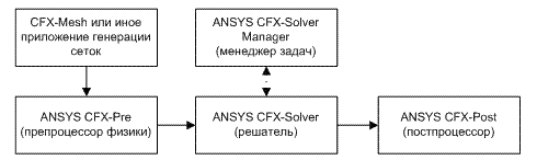Рис. 1Схема постановки и решения задачи с использованием пакета ANSYS CFX.

Рассмотрим, за какие этапы процесса постановки и решения задачи отвечает каждое приложение пакета.

CFX — Mesh, или другое приложение генерации сетки – это первый шаг постановки задачи. На данном этапе происходит следующее:

• определение геометрии области исследования;
• создание областей потоков жидкостей или газов, твердых областей и задание имен граничным областям;
• установка параметров сетки.

Система ANSYS CFX позволяет импортировать геометрические данные из большинства современных систем автоматизированного проектирования (CAD) и автоматически сгенерировать сетку на их основе. Таким образом, первый этап постановки задачи может быть выполнен во внешнем приложении (CAD-системе).

ANSYS CFX — Pre реализует процесс определения физики задачи. Физический препроцессор импортирует сетку, созданную на первом шаге. Это второй шаг постановки задачи, на котором определяются физические модели, на основе которых будет происходить симуляция процесса, а также их основные параметры и характеристики. CFX-Pre позволяет определить граничные условия процесса (входные, выходные параметры), модели теплообмена.

ANSYS CFX-Solver – это программа, реализующая процесс решения задачи вычислительной гидродинамики. Импортируется задача, поставленная посредством ANSYS CFX — Pre и производится поиск решения всех требуемых переменных:

• уравнения в частных производных интегрируются по всему объему задачи в области исследования, соответствует применению закона сохранения (масс или момента) к каждой исследуемой области;
• полученные интегральные уравнения преобразуются в систему алгебраических уравнений путем аппроксимирования членов в интегральных уравнениях;
• алгебраические уравнения решаются численным методом.

ANSYS CFX-Solver Manager – это надстройка над CFX-Solver. Она позволяет контролировать ход решения задачи:

• определять входные файлы решателя;
• запускать или приостанавливать CFX — Solver ;
• контролировать процесс решения задачи;
• устанавливать CFX — Solver для проведения параллельных вычислений.

ANSYS CFX-Post – это программа, предназначенная для анализа, визуализации и представления результатов, полученных в ходе решения задачи посредством ANSYS CFX-Solver. Для этого используются следующие средства:

• визуализация геометрии и исследуемых областей;
• векторные графики для визуализации направления и величины потоков;
• визуализация изменения скалярных величин (такие как температура, давление) внутри исследуемой области.

Графики, изображения и видео, полученные в результате анализа решения задачи можно сохранить в виде отдельных файлов.

2. Типы файлов ANSYS CFX

2.1 Общая схема обмена файлами

В процессе постановки, решения и анализа задачи, различные модули пакета ANSYS CFX обмениваются информацией посредством импорта/экспорта различных файлов.

Рис. 2Схема файлов, генерируемых в процессе постановки и решения задач программами из пакета ANSYS CFX.

Рассмотрим базовые файлы, посредством которых реализован процесс решения задач в пакете ANSYS CFX.

2.2 Файлы программы ANSYS CFX- Pre

Пакетный файл ANSYS CFX — Pre (*.cfx) содержит данные о физике процесса, и используется совместно с GTM -файлом, содержащем «базу данных» процесса симуляции. Эта пара файлов используется для сохранения и возобновления процесса постановки задачи в приложении ANSYS CFX — Pre. Пакетный файл – бинарный, вследствие чего непосредственное его редактирование невозможно.

Файлы GTM (» Geometry, Topology and Mesh» – «Геометрия, Топология и Сетка») содержат информацию о всех областях и сетках, требуемых для симуляции. Когда происходит импорт сетки в приложение ANSYS CFX — Pre, происходит формирование соответствующего GTM -файла. Таким образом, после импорта сетки, первоначальный файл, содержащий сетку, более не требуется. Эти файлы можно открывать непосредственно в среде ANSYS CFX — Post для детального анализа сеток.

Файл постановки задачи ANSYS CFX (*.def) содержит полную информацию о поставленной задаче, включая геометрию, сетку поверхности, граничные условия, параметры среды, параметры решателя и начальные переменные. Он создается ANSYS CFX — Pre и импортируется ANSYS CFX — Solver для запуска процесса решения задачи.

Файл CCL (» Command Language File» – «Файл языка команд») – это текстовый файл, описывающий постановку задачи решателю ANSYS CFX-Solver. Он может быть как сгенерирован отдельно, так и получен из файла постановки задачи, посредством применения утилиты cfx5cmds.

2.3 Файлы программы ANSYS CFX- Solver

Файл результатов ANSYS CFX — Solver (*.res) содержит полную информацию о результатах решения задачи, включая пространственную сетку и решения потоков жидкостей и газов. Он подобен файлу постановки задачи (*.def), но в дополнение к информации, содержащейся в файле постановки задачи, он еще содержит вычисленные значения каждой переменной в каждом узле сетки. Этот тип файлов может быть использован как входной файл ANSYS CFX — Pre, для определения начальных значений переменных для дальнейшего анализа.

Выходной файл ANSYS CFX — Solver (*.out) – это форматированный текстовый файл, содержащий информацию о настройках модели ANSYS CFX, состоянии решения в процессе работы ANSYS CFX — Solver и статистику выполнения задания.

2.4 Файлы программы ANSYS CFX- Post

ANSYS CFX-Post может обрабатывать файлы GTM (*.gtm) и файлы постановки задачи (*.def) (для детального изучения и выявления возможных проблемных сегментов сетки) а также файлы результатов (*.res) (для анализа и визуализации результатов решения поставленной задачи). В качестве результата работы, ANSYS CFX-Post генерирует различные графические файлы, содержащие графическое представление решения поставленной задачи.

3. Процесс постановки и решения типовой задачи посредством пакета ANSYS CFX

3.1 Постановка задачи

Рассмотрим одну из типовых задач, решаемых посредством пакета ANSYS CFX. В качестве примера, возьмем задачу смешения жидкостей с разными температурами, текущих по трубам. Пакет ANSYS CFX, по умолчанию, не содержит встроенных средств для построения геометрии. В качестве исходных данных могут быть использованы сетки, сгенерированными различными внешними приложениями генерации сеток (CAD -пакетами). В нашем случае есть 2 возможных пути получения сетки: либо использовать уже имеющуюся сетку, либо смоделировать новую сетку посредствам приложений, входящих в состав пакета ANSYS. Собственноручно создадим геометрию исследуемой области и сформируем сетку на ее основе.

Для описания геометрии исследуемой области воспользуемся приложением ANSYS DesignModeler. Это приложение, входящее состав пакета ANSYS Workbench, предназначенное для создания и редактирования геометрии. Создадим простую систему, состоящую из пары соединенных труб: основной трубы, и побочной трубы, по которой подается подогретая вода. Для этого создадим систему из двух цилиндров: больший представляет собой участок основной трубы, а меньший – «впайку» (Рис. 3).

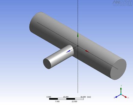
Рис. 3Постановка геометрии задачи.

Созданный нами файл геометрии экспортируем в генератор сеток ANSYS CFX — Mesh. Устанавливаем требуемые параметры точности сетки и получаем следующее представление исследуемой области (Рис. 4).

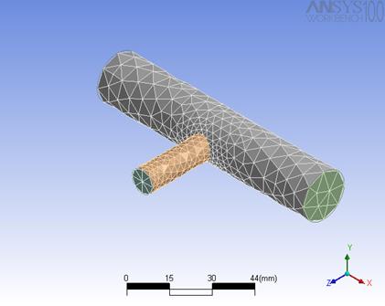
Рис. 4Формирование сетки на основе геометрии.

Сформированная сетка относительно грубая, но, как можно заметить из рисунка, плотность ее узлов непостоянна и значительно увеличивается в точке сочленения труб, что позволяет более детально исследовать интересующий нас участок.

Созданную сетку импортируем в ANSYS CFX — Pre и определяем физику задачи. Устанавливаем, что в данной системе будет находиться вода, задаем ее скорости и температуры на входах труб, указываем выход основной трубы (Рис. 5).

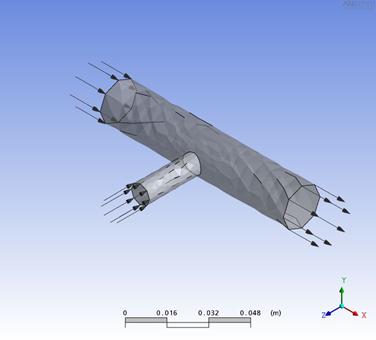
Рис. 5Определение физики задачи.

3.2 Решение и анализ задачи

В результате действий, описанных в 3.1, мы получили файл постановки задачи, который передается в ANSYS CFX — Solver Manager. В нем мы задаем параметры решения поставленной задачи (решение будет производиться на локальной машине, без применения параллельных вычислений) и запускаем процесс решения задачи посредством ANSYS CFX — Solver.

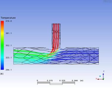
Рис. 6Картина потока воды в трубах.

Решение задачи на кластере происходит несколько по-другому. Требуется скопировать сгенерированный файл постановки задачи (*.def) на кластер, и запустить решение задачи следующим образом:

cl-run -as cfx13 -np 32 cfx_test -def. /test-file.def (более подробно о запуске см. в инструкции)


После запуска приведенной выше команды, будет запущен процесс решения задачи, поставленной в файле test-file.def. Решение будет производиться на 32-и ядрах, что определяется параметром -np 32. Результаты расчетов (файл с расширением *.res) появятся в той же директории, из которой производился запуск расчета. Файл *.res требуется скопировать на локальный компьютер, где и будет производиться анализ решения задачи посредством программы ANSYS CFX — Post.

В результате решения задачи мы получаем файл результатов, в котором храниться вся информация о потоках воды в рассматриваемой задаче. Для визуализации и анализа результатов, воспользуемся приложением ANSYS CFX — Post. После импорта результатов в приложение создадим 2 потока, соответствующих течению воды в основной и побочной трубе. Цвет потока установим соответствующим температуре воды. В результате, получим наглядную картину течения воды в данной системе труб (Рис. 6).

• ME 566Computational Fluid Dynamics for Fluids Engineering

  DesignANSYS CFX STUDENT USER MANUAL Version 11

  Gordon D. StubleyDepartment of Mechanical Engineering,
  University of Waterloo

  G.D. Stubley 2008

  January 30, 2008

  1

• Contents

  Contents i

  Preface iii

  I Tutorial 1

  1 Overview of CFD Process 21.1 Example Problem . . . . . . . . .
  . . . . . . . . . . . . . . . . . . . . . . . . 21.2 Domain . . . .
  . . . . . . . . . . . . . . . . . . . . . . . . . . . . . . . . . .
  . . 21.3 Domain Descritization: Mesh . . . . . . . . . . . . . . .
  . . . . . . . . . . 31.4 CFD Flow Solver . . . . . . . . . . . . .
  . . . . . . . . . . . . . . . . . . . . . 41.5 Post-processing . .
  . . . . . . . . . . . . . . . . . . . . . . . . . . . . . . . . .
  8

  2 Tutorial Commands 102.1 Introduction to the GUI . . . . . . .
  . . . . . . . . . . . . . . . . . . . . . . 102.2 Commands for Duct
  Bend Example . . . . . . . . . . . . . . . . . . . . . 13

  II Additional Notes 30

  3 Geometry and Mesh Specification 313.1 Basic Geometry Concepts
  and Definitions . . . . . . . . . . . . . . . . . 313.2 Geometry
  Creation . . . . . . . . . . . . . . . . . . . . . . . . . . . . .
  . . . 323.3 Mesh Generation . . . . . . . . . . . . . . . . . . . .
  . . . . . . . . . . . . . . 34

  4 CFX-Pre: Physical Modelling 424.1 Domain . . . . . . . . . . .
  . . . . . . . . . . . . . . . . . . . . . . . . . . . . . 434.2
  Initialization . . . . . . . . . . . . . . . . . . . . . . . . . .
  . . . . . . . . . . . 464.3 Output Control . . . . . . . . . . . .
  . . . . . . . . . . . . . . . . . . . . . . . 474.4 Simulation Type
  . . . . . . . . . . . . . . . . . . . . . . . . . . . . . . . . . .
  474.5 Solver Control . . . . . . . . . . . . . . . . . . . . . . .
  . . . . . . . . . . . . 47

  5 CFX Solver Manager: Solver Operation 495.1 Monitoring the
  Solver Run . . . . . . . . . . . . . . . . . . . . . . . . . . .
  49

  i

• Contents ii

  6 CFX-Post: Visualization and Analysis of Results 526.1
  Conventions . . . . . . . . . . . . . . . . . . . . . . . . . . . .
  . . . . . . . . . 526.2 Objects . . . . . . . . . . . . . . . . . .
  . . . . . . . . . . . . . . . . . . . . . . 546.3 Tools . . . . . .
  . . . . . . . . . . . . . . . . . . . . . . . . . . . . . . . . . .
  . . 556.4 Controls . . . . . . . . . . . . . . . . . . . . . . . .
  . . . . . . . . . . . . . . . 56

  7 Frequently Asked Questions 577.1 Where are the ANSYS-CFX
  tutorial files? . . . . . . . . . . . . . . . . . . 577.2 How to
  use an existing mesh after modifying the geometry? . . . . . 577.3
  How to use an existing CFX-Pre model after modifying the mesh? .
  577.4 How is heat conduction modelled in a single domain? . . . . .
  . . . . . 577.5 Why is there only a few point values given when
  exporting data

  along a line normal to a wall? . . . . . . . . . . . . . . . . .
  . . . . . . . . . 587.6 How is a thin guide vane modelled? . . . .
  . . . . . . . . . . . . . . . . . . 58

• Preface

  In these notes the basic steps in a CFD solution will be
  illustrated using the pro-fessional software ANSYS Workbench
  Version 11which includes the componentsDesignModeler, Meshing, and
  Advanced CFD (all trademarks of ANSYS). Thesenotes include an
  introductory tutorial and a mini users guide. In particular,
  thenotes are pertinent to the simulation of two dimensional steady
  incompressiblelaminar and turbulent fluid flows on stationary
  meshes. They are not meant to re-place a detailed users guide. For
  full information on these components refer to theon-line help
  documentation provided with the software 1.

  These notes include sections on:

  Overview of CFD Simulation An introductory section outlining the
  componentsof a CFD simulation. Includes the description of an
  example CFD analysisproblem;

  Commands for the Example Problem: A complete step-by-step list
  of instructionsfor solving the example problem.

  Software Components: A description of the concepts and operation
  involved inthe five software components: DesignModeler, Meshing,
  CFX-Pre, CFX-Solver, and CFX-Post; and

  Frequently Asked Questions: Suggestions for further study and
  for solving typi-cal flow cases.

  The following font/format conventions are used to indicate the
  various com-mands that should be invoked:

  Menu/Sub-Menu/Sub-Sub-Menu Item chosen from the menu hierarchy
  at the top of amain panel or window,

  Button/Tab Command Option activated by clicking on a button or
  tab,

  Link description Click on the description to move by a link to
  the next step/page;

  Name val ue Enter the val ue in the named box,

  1Many of the features available in these software components
  will not be explored in introductoryCFD courses.

  iii

• PREFACE iv

  Name selection Choose the selection(s) from the named list,Name
  Panel or window name,

  Name On/off switch box, and Name On/off switch circle (radio
  button).

• Part I

  Tutorial

  1

• Chapter 1

  Overview of CFD Process

  1.1 Example Problem

  To provide a context for these notes consider the application of
  CFD to studyingthe flow in a short radius bend within the duct
  system shown in Figure 1.1. Thereis a flow of water upwards into
  the bend.

  The side view of the duct bend geometry is shown in Figure 1.2.
  The radiusof the inner wall bend is R1= 0.025[m]. The spacing
  between the duct inner walland outer wall is H3= 0.1[m]. The duct
  has a width (into the page) of 1[m]. Theaverage speed of the water
  flow through the duct is 3[m/s].

  The purpose of the CFD analysis is to determine if and where
  flow separation isan issue. CFD is well suited to this task because
  it can provide a detailed representa-tion of the velocity and
  pressure fields throughout the flow domain. By examiningthe
  velocity field it will be possible to identify regions where the
  flow separates andreverses direction and by examining the pressure
  field it will be possible to identifyregions where flow reversal is
  likely to occur. In this chapter a brief description ofhow these
  field properties are determined is presented.

  1.2 Domain

  The CFD simulation is restricted to a specific three dimensional
  region known asthe domain. For the duct bend example, the domain,
  shown in Figures 1.1 and 1.2,is a thin volume that is bounded by
  the outer wall, the inner wall, by planes per-pendicular to the
  flow upstream and downstream of the bend, and by surfaces inthe x y
  plane on the front and back sides. The domain extends V 2= 0.1[m]
  up-stream from the bend and H4= 0.25[m] downstream from the bend.
  The domainis 0.02[m] wide.

  The geometry of the domain is represented in digital form by
  solid modellingsoftware. The resulting geometric model is known as
  a solid or solid-body for his-torical reasons. The volume of the
  solid geometric model is the volume where thefluid flow is
  modelled.

  2

• CHAPTER 1. OVERVIEW OF CFD PROCESS 3

  xz

  y

  CFD Domain

  Figure 1.1: Schematic of the region near a short radius bend in
  a duct system. Wateris flowing upwards into the bend and to the
  right out of the bend. A wireframerepresentation of the CFD flow
  domain is also shown.

  1.3 Domain Descritization: Mesh

  It is not possible to analytically determine mathematical
  functions for the variationof velocity and pressure throughout
  complex domains. Therefore approximate val-ues of the velocity
  components, Ui , i = 1,2,3,

  1 and pressure, p, are generated onlyat discrete points or nodes
  throughout the domain. The locations of the nodes arebased on a
  mesh. A mesh for the duct bend geometry is shown in Figure 1.3.

  The mesh is comprised of a set of relatively simple three
  dimensional polyhedralelements. The example mesh is comprised of
  hexahedral elements. For all meshes,the set of elements is
  non-overlapping, fills the domain, and fits the boundaries ofthe
  domain. For CFX meshes, the nodes are located at the vertices of
  the elements.The example mesh is only one element thick in the z
  direction and the surfacemeshes on the front and back surfaces are
  identical. This is suitable for this flowbecause there is no
  significant variation of flow properties in the z direction.

  1Index notation is used in these notes, where the x,y, and z
  directions are indicated by indices 1,2,and 3 respectively.

• CHAPTER 1. OVERVIEW OF CFD PROCESS 4

  Figure 1.2: Solid body model of the duct bend geometry included
  in the CFD flowdomain.

  1.4 CFD Flow Solver

  CFD software assumes that each node is surrounded by a finite
  control volumebounded by planar faces as illustrated in Figure 1.3.
  By applying the principles ofconservation of momentum and mass to
  each control volume, a set of finite volumeequations are formed
  which can be solved to provide nodal values of velocity
  andpressure.

  After a mesh has been generated, there are three major steps to
  create a simula-tion of the velocity and pressure fields on the
  mesh:

  Flow Model Specification: identify all significant flow
  processes (such as advectiveflows and stress tensor forces) and
  their appropriate models;

  Finite Volume Equation Generation: apply a set of numerical
  approximations toestimate all control volume flow processes in
  terms of the nodal field propertyvalues. When applied to the
  conservation principles, this leads to a set of finitevolume
  equations; and

  Finite Volume Equation Solution: use a nonlinear matrix solution
  algorithm tosolve the equation set for estimates of the nodal
  values of velocity and pres-sure.

• CHAPTER 1. OVERVIEW OF CFD PROCESS 5

  Figure 1.3: Mesh of hexahedral elements for the duct bend
  geometry showing atypical node and finite control volume.

  By convention the software that performs these three steps is
  referred to as the CFDflow solver.

  Flow Model Specification

  The first step of the CFD flow solver requires input from the
  CFD analyst to iden-tify the relevant flow processes and to choose
  suitable models for these processes.

  For the example problem of flow through the duct bend:

  Type of Flow: the flow is modelled as turbulent, non-buoyant,
  steady in themean flow properties, and doesnt involve heat
  transfer;

  Fluid Type and Properties: the fluid, water, is modelled as a
  constant propertyNewtonian liquid, with a density of = 1000[k g/m3]
  and dynamic viscosityof = 0.001[Pas];

  Flow Domain Properties: the domain is modelled as
  stationary;

  Turbulence Model: the mean action of the turbulent eddying
  motion onthe mean velocity field is accounted for with the
  k-epsilon (k «) model. In

• CHAPTER 1. OVERVIEW OF CFD PROCESS 6

  this model, the turbulent Reynolds stresses, u i u j , are
  related to the meanvelocity strain rate by

  u i u j t Ui x j

  + Uj xi

  !where the turbulent viscosity, t , is proportional to the fluid
  density, thevelocity scale (intensity) of the turbulent eddies, and
  the length scale of theeddies. The scales of the turbulent eddying
  motion are estimated from twofield properties of the turbulence
  which are calculated at each node: k, meanturbulent kinetic energy
  (i.e. kinetic energy associated with swirling turbu-lent eddies)
  and «, the rate at which k is dissipated by molecular action;
  and

  Boundary Conditions: modelling the influence of the surroundings
  on theflow domain are specified for each surface on the flow domain
  and are mod-elled as:

  [Inflow Surface:] with a uniform normal velocity of Vin =
  3[m/s],

  turbulent intensity, I pk

  Vin= 5%, and turbulent length scale, l k 32

  «=

  0.01[m]; [Outflow Surface:] with a uniform relative pressure of
  0[Pa]; [Inner and Outer Walls:] modelled as smooth no-slip walls.
  The tur-

  bulent wall shear stress is estimated with the Law of the Wall
  for equi-librium turbulent boundary layers;

  [Front and Back Surfaces:] modelled as symmetry surfaces
  implyingno mass flow across these surfaces and all normal gradients
  are zero.

  Finite Volume Equation Generation

  As mentioned above, a finite control volume surrounds each node
  in the mesh.Once calculated the nodal field values are
  representative average values for theirrespective control volumes.
  To calculate the nodal field values a set of discrete alge-braic
  equations based upon conservation principles are formed. For the
  duct bendexample, these equations are based on conservation of
  mass, momentum in 3 direc-tions, x, y, and z, turbulent kinetic
  energy, and its dissipation rate.

  The finite volume methodology can be illustrated with a
  simplified discussionof the generation of the discrete mass
  conservation equation. Consider mass conser-vation for the control
  volume surrounding the P node shown in Figure 1.3. Withthe
  specified steady incompressible flow model, mass conservation
  implies that thesum of mass flows across the faces of the P control
  volume must balance or

  0=faces

  ~Vface nAface (1.1)

  where ~Vface is the face average velocity, n is the face
  outwards pointing unit normalvector, and Aface is the face area.
  Notice that Equation 1.1 provides a relationship in

• CHAPTER 1. OVERVIEW OF CFD PROCESS 7

  terms of face velocities and not one in terms of the nodal
  velocities. However, eachinterior face separates two neighbour
  nodes. If numerical interpolation functionsare used to estimate the
  face velocities in terms of the neighbour nodal values thena useful
  discrete mass conservation equation can be formed in terms of the
  nodalvalues.

  Typically the interpolation functions assume some form of linear
  interpolation.While largely prescribed by the CFD software, the
  choice of certain interpolationfunctions can be set by the CFD
  analyst.

  For the duct bend example the following interpolation functions
  are specified:

  Mass flows: linear-linear-linear interpolation;

  Diffusive flows: linear-linear-linear interpolation;

  Advective flows: upwind weighted linear interpolation based on
  nodal values andgradient estimates (high resolution scheme)

  Pressure forces: linear-linear-linear interpolation; and

  Stress tensor forces: linear-linear-linear interpolation.

  Finite Volume Equation Solution

  For the duct bend example, there are five unknown field
  properties at each node,pressure, three velocity components,
  turbulent kinetic energy, and its dissipationrate. As explained
  above, five corresponding discrete algebraic equations can
  begenerated for each node based on conservation of mass, momentum
  in three di-rections, turbulent kinetic energy, and its dissipation
  rate. Therefore, once finitevolume equations are generated for each
  node there is a set of equations which canbe solved to determine
  estimates of the nodal field properties.

  This equation set is highly coupled, both linearly and
  nonlinearly. Therefore aniterative solution algorithm is
  implemented in the CFD solver to obtain estimatesof the nodal field
  properties. The essence of the algorithm:

  1. Make an initial guess for each field property at each
  node;

  2. Determine the imbalance, residual, in each finite volume
  conservation equa-tion. If the residual imbalance values are
  sufficiently small stop the iteration.If not continue with the
  following:

  3. Use the residual values to estimate improved values for the
  nodal field prop-erty values;

  4. Return to Step 2.

• CHAPTER 1. OVERVIEW OF CFD PROCESS 8

  Figure 1.4: Vector plot of the simulated flow field through a
  duct bend showingseparated flow on the inner wall downstream of the
  bend.

  1.5 Post-processing

  The CFD flow solver provides estimates of fundamental field
  properties at eachnode. Often this information is insufficient. For
  example, in the duct bend flow itis necessary to know the extent of
  the possible separated flow regions and the dropin total pressure
  through the bend. This information is found by post-processingthe
  nodal values to provide graphic images or to calculate secondary
  values of directrelevance to evaluating the flow.

  Figure 1.4 shows a vector plot of the simulated flow through the
  duct bend. Aseparated flow region adjacent to the inner wall
  downstream of the bend is clearlyseen. Regions of high speed and
  low speed flow are also seen in this visualization.

  A summary of the complete CFD model including meshing details is
  shown inFigure 1.5.

• CHAPTER 1. OVERVIEW OF CFD PROCESS 9

  Figu

  re1.

  5:Su

  mm

  ary

  ofth

  eC

  FDm

  odel

  for

  flow

  thro

  ugh

  adu

  ctbe

  nd.

• Chapter 2

  Tutorial Commands

  2.1 Introduction to the GUI

  Windows XP/NEXUS

  The CFD software is available on the workstations in the
  Engineering Comput-ing labs, Fulcrum (E2-1313), Wedge (E2-1302B),
  Helix (RCH-108), and WEEF (E2-1310), and the Mechanical Engineering
  4th year computing room, E3-3110. Theworkstations use the Windows
  XP operating system on Waterloo NEXUS. Youshould be familiar with
  techniques to create new folders (or directories), to deletefiles,
  to move through the folder (directory) system with Windows
  Explorer, toopen programs through the Start menu on the Desktop
  toolbar, to move, resize,and close windows, and to manage disk
  space usage with tools like WinZip.

  Introduction to Workbench

  The ANSYS Workbench environment provides an interface to manage
  the filesand databases associated with the individual software
  components. These files anddatabases are organized into a
  particular project. To get a feel for this environ-ment and the
  GUIs associated with the software components, we will look at
  apre-prepared project on flow through a pipe bend.

  1. Create a working directory called CFDTest on your N
  drive.

  2. Use a web browser to visit the UW-ACE ME 566 course page
  (uwace.uwaterloo.ca).Under the Lessons tab and open the Student
  User Manual folder. Click on thelink to PipeBend.zip and follow the
  instructions to download the archive con-taining the working
  files.

  3. Use WinZip to extract the files in the PipeBend archive into
  your workingdirectory.

  4. Open ANSYS Workbench fromStart/Programs/Engineering/ANSYS
  11.0/ANSYS Workbench.

  10

• CHAPTER 2. TUTORIAL COMMANDS 11

  5. Open the project file. Check that Open: Workbench Project is
  selected be-fore using the Browse button below the Open: Workbench
  Projects panel areato find and selecting the file PipeBend.wbdb
  from your working directory.

  6. There are three main areas on the screen: command menus,
  buttons, and tabsat the top, a list of potential Project Tasks on
  the left, and a list of the fileslinked to the project.

  7. On-line help for Workbench, DesignModeler, and CFX-Mesh is
  available inweb-page format similar to other Windows programs.
  Choose Help/ANSYSWorkbench Help to open the ANSYS Workbench
  Documentation. Search forkeyword Tutorials and select CFX-Mesh
  Help. Follow the Tutorials link to seethe list of available
  tutorials.

  Introduction to DesignModeler/CFX-Mesh GUI

  1. In the Workbench file area click on the item name PipeBend
  just to the rightof the DesignModeler button ( DM ). Notice that
  the Project Tasks area atthe left adjusts to reflect your choice.
  Under DesignModeler Tasks chooseOpen to open the geometry file.

  2. A new page for DesignModeler will open. Go back to the
  Project page byclicking on the PipeBend [Project] tab at the top
  left of the screen. Click on

  the PipeBend [DesignModeler] tab to return to the DesignModeler
  page.

  3. There are four major areas on the page: command menus and
  buttons atthe top, a Tree View and Sketch Toolbox on the left, a
  Details View at thebottom left, and a Model View window. Place the
  mouse cursor over oneof the command buttons in the top row. A brief
  description of the buttonsaction should appear (you may need to
  click in the window once to make itactive). Visit each button with
  the mouse cursor to see its action.

  4. One method of controlling the view is with the coordinate
  system triad inthe lower right corner of Model View. Click on the Z
  axis of the triad to seea back view of the pipe bend. Click on the
  cyan sphere to select the isometricview.

  5. Another method of controlling the view is with the mouse left
  button inconjunction with a mouse action selection. From the upper
  row of buttons,select the Pan action. Holding the left mouse button
  down, drag the mouse

  over the Model View to translate the view. Select the Zoom
  action andrepeat with an up-down mouse action to change the size of
  the view.

  6. Select the Rotate action. The rotate action is context
  sensitive in that itdepends upon the position of the mouse cursor.
  With the mouse cursor closeto the pipe bend, press the left mouse
  button to get free 3D rotation. The point

• CHAPTER 2. TUTORIAL COMMANDS 12

  of rotation can be changed by clicking the left button while the
  cursor is onthe pipe bend surface (this may take some
  experimentation). With the mousecursor in a corner of the Model
  View, press and hold the left mouse buttonto get a roll action in
  which there is 2D rotation about an axis perpendicularto the Model
  View window. Move the cursor to either the left or right ofthe
  Model View and hold the left button to get a yaw action in which
  thereis 2D rotation about the vertical axis. Move the cursor to
  either the top orbottom of the Model View and hold the left button
  to get a pitch action inwhich there is 2D rotation about the
  horizontal axis.

  7. Rotate, zoom, and pan actions can be achieved directly by
  pressing the middlemouse key alone, with the Shift key, and with
  the Ctrl key, respectively.

  8. The Tree View on the left shows the geometric entities that
  were used togenerate the cylinder. Expand the 1 Part, 1 Body entity
  and click on Solid tosee some properties of the cylinder in the
  Details View. The pipe bend wasgenerated from two entities:

  a) Sketch1: which can be found in the Plane4 entity. Click on
  Sketch1 tohighlight the circle that the pipe bend is based upon
  with yellow.

  b) Sketch2:. which can be found in the YZPlane entity. Click on
  the Sketch2to highlight the path that is swept out by Sketch1 to
  generate the pipebend.

  9. In the help page search for keywords rotation modes and
  select «Rotation Cur-sors in the Rotate Mode» to find more
  information on changing the view.

  10. Click the X button on the PipeBend [DesignModeler] tab to
  close the De-signModeler page. You can click No to quit without
  saving changes.

  Introduction to the Advanced CFD GUI

  The tasks associated with CFD simulation in Workbench are
  referred to as Ad-vanced CFD Tasks. For historical reasons, the GUI
  for the three Advanced CFDTasks is slightly different from that of
  the other Workbench components. We willuse CFX-Post to look at the
  completed simulation of flow through a pipe bend toget a feel for
  these differences.

  1. In the Workbench file area click on the item name
  PipeBend_001. Under Ad-vanced CFD Tasks, choose Open in CFX-Post to
  open the results file (PipeBend_001.res).All of the pertinent CFD
  model data (mesh, flow attributes, and boundarycondition
  information) for this problem is stored in this file.

  2. A new page for CFX-Post will open.

  3. There are three major areas on the screen: Command menus and
  buttons atthe top, outline and detail panels on the left, and 3D
  Viewer window. Wire-frame models of the pipe inlet and outlet
  should be in the Viewer. To see the

• CHAPTER 2. TUTORIAL COMMANDS 13

  pipe bend click the Domain 1 Default object on in the tree under
  PipeBend_OO1and Domain 1 in the Outline panel.

  4. The mouse button action for controlling the view is similar
  to that in Design-Modeler.

  5. The coordinate system triad is shown in the lower right
  corner. Unlike inDesignModeler, the triad cannot be used to change
  the view. To set standarddirectional views type x, y, or z while
  the Viewer window is active to getviews in the positive axis
  directions and type X, Y, or Y to get views in thenegative axis
  directions. Other standard key mappings can be seen by clickingon
  the Show Help Dialog icon at the right of the lower row of icon
  buttons.

  6. On-line help is available, Help. Open the main table of
  contents, Help/MasterContents. Context-sensitive help is also
  available. Right click on Default Legend View 1object and choose
  Edit. Position the mouse pointer in the Details of DefaultLegend
  View 1 panel and press to bring up the help page for that
  panel.

  7. This should give a sense of the operation of the Advanced CFD
  GUI. Whenyou have finished, return to the Workbench Project page.
  Exit by File/CloseProject and choose No: do not save any items.

  8. Clean up by deleting the CFXTest directory.

  2.2 Commands for Duct Bend Example

  To set-up the project files and options:

  Create a new folder N:/Ductbend1 to be the working directory for
  the projectfiles.

  Open ANSYS Workbench fromStart/Programs/Engineering/ANSYS
  11.0/ANSYS Workbench. To open a new project:

  1. In the Start window, select Empty Project in the New
  panel,

  2. From the menu bar choose File/Save As … to create a project
  file in yourworking directory, and

  3. In the Save As window fill in File name: Ductbend.wbdb and
  click the

  Save button.

  From the menu bar choose Tools/Options … to set the length
  units and meshingtool options:

  In the Options window expand the + DesignModeler entity and

  1When NEXUS network traffic is high, it is better to make the
  working directory on your localmachine, i.e. C:/Temp/Ductbend.

• CHAPTER 2. TUTORIAL COMMANDS 14

  * Select Units in the tree view on the left to set Length Unit
  Meter ;and

  * Select Grid Defaults (Meters) in the tree view on the left to
  setMinimum Axes Length 0.5 and Major Grid Spacing 0.1 .

  Expand the + Meshing entity and select Meshingto Set Show
  Mesh-ing Options Panel at Startup No , Default Physics Preference
  CFD , and

  Default Method Automatic (Patch Conforming/Sweeping) .

  Expand the + Common Setting entity and select Geometry Import
  to:

  * set Named Selection Processing Yes ; and

  * set Named Selection Prefixes (i.e. leave blank).

  Click OK to save the options and close the window,

  Geometry Model

  The commands listed below will use DesignModeler to create a
  solid body geometrythat will represent the flow domain.

  Under Create DesignModeler Geometry, choose New Geometry,

  Check that the desired length unit is Meter is selected and
  click Ok in theunits window that appears,

  In the Tree View, select the XYPlane entity and then click the
  New Sketchicon to create the Sketch1 entity as a component of the
  XYPlane.

  To start the sketching , select the Sketching tab and click on
  the Z coordinateof the triad in the lower right corner of the Model
  View, and draw in the 2Dsketch of the flow path;

  1. Select the Draw toolbox and use the Arc by Center tool to
  sketch theinner wall bend shape:

  a) Place the cursor over the origin (watch for the P constraint
  symbol)and left mouse button click.

  b) Move the cursor to the left along the X axis. With the C
  constraintvisible click the left mouse button to put the start
  point of the arcon the X axis.

  c) Sweep the cursor clockwise until the C constraint appears at
  the Yaxis. Click the left mouse button.2

  2. Switch to the Dimensions toolbox to size the inner wall bend
  radius:

  2Notice that the drawing instruction steps are provided in the
  lower left corner.

• CHAPTER 2. TUTORIAL COMMANDS 15

  a) Select the Radius tool;b) Select a point on the arc. Then
  move the cursor to the inside of the

  arc near the origin. Click to complete a dimension which is
  labelledR1.

  c) In the Details View notice that R1 is shown under the
  Dimensionstitle.

  d) Change the value of R1 to 0.025 [m]. Notice the arc radius
  changesautomatically. If the dimension is poorly placed on your
  sketch youcan use the Move tool to correct the placement.

  3. Switch back to the Draw toolbox to sketch the inner entrance
  wall:

  a) With the Line tool selected, place the cursor in the lower
  left quad-rant of the XY plane near the arc. Click the left mouse
  button.Move the mouse cursor down to create a vertical line. Look
  for theV constraint symbol and click the left mouse button;

  b) Switch to the Dimensions toolbox to size the inner entrance
  walllength:

  i. Select the General tool;ii. Select a point near the centre of
  the line. Click and drag the

  cursor to the right to form the dimension lines. Release
  themouse button where the label, V2, is to be placed.

  iii. In the Details View change the value of V2 to 0.10 [m].c)
  To join the inner entrance wall and the inner wall bend switch
  to

  the Constraints toolbox;

  i. Select the Coincident tool;ii. Select the upper end of the
  entrance inner wall with a left

  mouse button click. The square end marker should be yellow;iii.
  Select the square end marker of the arc that lies on the X axis

  with a left mouse button click. The inner entrance wall
  shouldjoin the inner wall bend.

  4. To draw a line across the inflow (entrance):

  a) Use the Line tool in the Draw toolbox;b) Place the cursor
  over the bottom end point of the entrance inner

  wall and notice that a P constraint symbol appears. Left
  mousebutton click to select this point and then move the cursor to
  theleft and click while the H constraint symbol is visible.

  c) Use the General tool in the Dimensions toolbox:d) Select a
  point near the centre of the line. Click and drag the cur-

  sor to the bottom to form the dimension lines. Release the
  mousebutton where the label, H3, is to be placed.

  e) In the Details View change the value of H3 to 0.1 [m].

• CHAPTER 2. TUTORIAL COMMANDS 16

  5. Repeat the procedure used for the entrance inner wall to draw
  the exitinner wall:

  a) Draw a horizontal line in the upper right XY quadrant near
  the endpoint of the inner wall bend;

  b) Set the length of the line to 0.25 [m] with the General tool
  from

  the Dimensions toolbox;

  c) Join the exit inner wall to the inner wall bend with the
  Coincident

  tool from the Constraints toolbox.

  6. Draw the outer entrance wall with the Line tool. Start at the
  outer(left) end point of the inflow edge (look for the P constraint
  symbol)and draw a vertical line that is coincident (C) with the X
  axis;

  7. Draw the outer bend wall with the Arc by Center tool. Put the
  centreat the origin, make the start point at approximately 20 above
  the X axisin the upper left quadrant, and make the end point
  coincident (C) withthe Y axis. Use the Coincident constraint tool
  to join the start pointof the arc to the end point of the outer
  entrance wall;

  8. Draw the outer exit wall with the Line tool. Draw a
  horizontal (H)line coincident (C) with the Y axis above its final
  desired location. Usethe Coincident constraint tool to join this
  line to the end of the outer

  bend wall. Use the Equal Length constraint tool to make the
  outer exitwall the same length as the inner exit wall; and

  9. Draw a line from the end of the outer exit wall to the end of
  the innerexit wall to form the outflow edge. Make sure that the end
  points arecoincident (P).

  The sketch should now be an enclosed contour on the XYPlane.

  To create the three dimensional solid body:

  1. Switch to the Tree View by selecting the Modeling tab;

  2. Click on the Extrude button to create the Extrude1 feature .
  In theDetails View:

  Check Base Object Sketch1 ,

  Select Operation Add Material , Select Direction Vector None
  (Normal) , Set FD1, Depth (> 0) 0.02 ,

  Select As Thin/Surface? No , and Select Merge Topology? No .

• CHAPTER 2. TUTORIAL COMMANDS 17

  3. Click on the Generate button to create a Solid. Use the
  isometric viewin the Model View to check that you have a three
  dimensional solid greybody.

  Name the faces of the solid body to make it easy to apply
  boundary condi-tions:

  Choose Tools/Named Selection.

  In the Details panel set Named Selection Outflow ;

  In the Graphics View select the outflow face (or surface) and
  then clickGeometry Apply in the Details View;

  Click on the Generate button to complete the named selection
  process;

  Repeat for surfaces named Front, Back, InnerWall, OuterWall, and
  In-flow. Some faces, like InnerWall and OuterWall, may be composed
  ofthree primitive surfaces. To select a set of faces hold the
  «Ctrl»key downwhile clicking on the component faces in the Graphics
  View.

  Save an image of the geometry by clicking on the Image Capture
  (camera)

  button. Set File name: Geometry to save the png format file.

  Choose File/Save As … and set File name: Ductbend.agdb in the
  Save As win-

  dow. Click Save to close window.

  Return to the Project page by clicking on the Ductbend [Project]
  tab at thetop left corner of the window.

  ANSYS Mesh Generation

  The commands listed below use ANSYS swept mesher3 to generate a
  discrete hexa-hedral mesh in the flow domain:

  Choose the New Mesh DesignModeler Tasks; Notice the three
  primary areas:Geometry View, Outline View, and Details View, in the
  Meshing window.

  In the outline view, right click on the Mesh entity and select
  Generate Mesh.Notice that a simple hexahedral mesh is generated
  with automatic settings.To achieve a realistic CFD simulation this
  mesh is modified by:

  1. Ensure that a structured hexahedral mesh is produced by:

  a) Select the Face Selection Filter icon from the button
  commandsat the top of the meshing window;

  b) Right click on the Mesh entity and select Insert/Mapped Face
  Meshing;

  3For CFX-Meshing tools see the section on CFX Mesh Generation,
  page 27.

• CHAPTER 2. TUTORIAL COMMANDS 18

  c) On the Geometry View select the Front face; and

  d) then click Geometry Apply in the Details View.

  2. Set the mesh one unit wide in the z direction by:

  a) Select the Edge Selection Filter icon from the button
  commandsat the top of the meshing window;

  b) Right click on the Mesh entity and select Insert/Sizing;c) On
  the Geometry View select one of edges between the front and

  back faces at the outflow and then click Geometry Apply in
  theDetails View;

  d) In the Details View set

  Type Number of Divisions

  Number of Divisions 1

  Edge Behaviour Hard

  Bias Type No Biase) right click on the Mesh entity and select
  Generate Mesh.

  3. Set the mesh spacing in the cross-stream direction so that it
  is fine nearthe walls and coarse in the core by:

  a) Right click on the Mesh entity and select Insert/Sizing;b) On
  the Geometry View select the front edge at the inflow between

  outer and inner walls and the front edge oat the outflow
  betweenthe walls (remember to use the «Ctrl» key) and then click
  Geometry

  Apply in the Details View;

  c) In the Details View set

  Type Number of Divisions

  Number of Divisions 25

  Edge Behaviour Hard Bias Type

  Bias Factor 50d) right click on the Mesh entity and select
  Generate Mesh.

  4. Set a uniform mesh spacing in the streamwise direction
  direction in theentrance region by:

  a) Right click on the Mesh entity and select Insert/Sizing;b) On
  the Geometry View select the front edges of the inner and outer

  walls in the entrance region and then click Geometry Apply in
  theDetails View;

  c) In the Details View set

  Type Element Size

• CHAPTER 2. TUTORIAL COMMANDS 19

  Element Size 0.01

  Edge Behaviour Hard

  Bias Type No Biasd) right click on the Mesh entity and select
  Generate Mesh.

  5. Set uniform mesh spacing in the streamwise direction
  direction in thebend region by:

  a) Right click on the Mesh entity and select Insert/Sizing;b) On
  the Geometry View select the front edge of the inner bend wall

  and then click Geometry Apply in the Details View;

  c) In the Details View set

  Type Number of Divisions

  Number of Divisions 20

  Edge Behaviour Hard

  Bias Type No Biasd) right click on the Mesh entity and select
  Generate Mesh.

  6. Set an expanding mesh spacing in the stream direction of the
  exit regionby:

  a) Right click on the Mesh entity and select Insert/Sizing;b) On
  the Geometry View select the front edges of the inner and outer

  walls in the exit region and then click Geometry Apply in the
  De-tails View;

  c) In the Details View set

  Type Element Size

  Element Size 0.01

  Edge Behaviour Hard Bias Type

  Bias Factor 5d) right click on the Mesh entity and select
  Generate Mesh.

  7. Save an image of the mesh by selecting New Figure or Image
  Image to Filefrom the icons above the graphics window. Set File
  name: Mesh to savethe png format file.

  8. Save the mesh with File/Save and set File name: Ductbend.cmdb
  ;

  9. Return to the Project page by clicking on the Ductbend
  [Project] tab atthe top left corner of the window.

• CHAPTER 2. TUTORIAL COMMANDS 20

  Pre-processing

  In this phase the complete CFD model (mesh, fluids, flow
  processes, boundaryconditions, etc.) is defined and saved in a
  hierarchical database.

  To accomplish these steps execute the following commands:

  Highlight the Mesh Model, Ductbend.cmdb, in the Project page and
  selectCreate CFD Simulation with Mesh under Advanced CFD Tasks;

  After a short wait the CFX-Pre page will open. This page is
  similar to the CFX-Post page. There are three main areas: the menus
  and command buttons atthe top, the Viewer window at the right, and
  the Outline view of the databasetrees at the left;

  To create a new material with the required water properties,
  right mouseclick on the Materials entity in the Outline tree and
  select Insert/Material. Inthe Insert Material panel, fill in Name
  Water nominal and click OK to open apanel with two tabs:

  Click the Basic Settings tab and set:

  Option Pure Substance , Material Group Constant Property Liquids
  , Material Description off, Thermodynamic State on and
  Thermodynamic State Liquid . Click the Material Properties tab and
  set:

  Option General Material , in the Equation of State area set,

  Option Value , Density 1000 k gm3 , expand Transport Properties
  + ,

  Dynamic Viscosity on and Dynamic Viscosity 0.001 Pa s ,and then
  click Ok .

  In the Outline view, right mouse click the Simulation Type
  entity and select Edit

  to open the Simulation Type panel. Check that Option Steady
  State is setand then click Ok .

  In the Outline view, double left mouse click the Default Domain
  entity to openthe Domain: Default Domain panel which will have
  several tabbed sub-panels.

• CHAPTER 2. TUTORIAL COMMANDS 21

  On the General Options sub-panel, set:

  * Location B28 and notice that the geometry is highlighted
  ingreen in the Viewer window,

  * Domain Type Fluid Domain ,* Fluids List Water nominal ,*
  Particle Tracking off,* Reference Pressure 1 atm ,* Buoyancy Option
  Non Buoyant , and* Domain Motion Option Stationary .

  on the Fluid Models sub-panel set:

  * Heat Transfer Model Option None ,* Turbulence Model Option
  k-Epsilon ,* Turbulent Wall Functions Option Scalable ,* Reaction
  or Combustion Model Option None , and* Thermal Radiation Model
  Option None ,

  on the Initialization sub-panel ensure that Domain
  Initialization is offand then click Ok to close the panel.

  To prepare for implementing the boundary conditions, expand the
  expand+ Ductbend.cmdb mesh model to see the Principal 2D Regions of
  the geometry.

  Check that all 2D regions are highlighted.

  Right mouse click Back and select Insert/Boundary to open the
  boundary de-tails panel. In this panel:

  under the Basic Settings tab set:

  * Boundary Type Symmetry , and* Location Back ,

  and then click Ok to close the panel and create the new boundary
  object.Notice that perpendicular red arrows appear on the back
  surface in the Viewerwindow and the boundary object is listed in
  the Default Domain entity. Clickingon back surface object in the
  Default Domain database causes the back surfacemesh to be outlined
  with green in the Viewer window. A double mouse clickwill re-open
  the boundary details panel.

  Right mouse click Front and select Insert/Boundary to open the
  boundary de-tails panel. In this panel:

• CHAPTER 2. TUTORIAL COMMANDS 22

  under the Basic Settings tab set:

  * Boundary Type Symmetry , and* Location Front ,

  and then click Ok to close the panel.

  Right mouse click Inflow and select Insert/Boundary to open the
  boundary de-tails panel. In this panel:

  under the Basic Settings tab set:

  * Boundary Type Inlet , and* Location Inflow ,

  and under the Boundary Details tab set:

  * Flow Regime Option Subsonic ,* Mass and Momentum Option Normal
  Speed ,

  * Normal Speed 3 ms1 ,* Turbulence Option Intensity and Length
  Scale ,* Value 0.05 ,

  * Eddy Length Scale 0.01 m ,

  and then click Ok to close the panel and create the new boundary
  object.

  Right mouse click inner wall and select Insert/Boundary to open
  the boundarydetails panel. In this panel:

  under the Basic Settings tab set:

  * Boundary Type Wall , and* Location InnerWall ,

  and under the Boundary Details tab set:

  * Wall Influence on Flow Option No Slip ,* Wall Velocity off,*
  Wall Roughness Option Smooth Wall ,

  and then click Ok to close the panel.

  Right mouse click OuterWall and select Insert/Boundary to open
  the boundarydetails panel. In this panel:

• CHAPTER 2. TUTORIAL COMMANDS 23

  under the Basic Settings tab set:

  * Boundary Type Wall , and* Location OuterWall ,

  and under the Boundary Details tab set:

  * Wall Influence on Flow Option No Slip ,* Wall Velocity off,*
  Wall Roughness Option Smooth Wall ,

  and then click Ok to close the panel.

  Right mouse click Outflow and select Insert/Boundary to open the
  boundarydetails panel. In this panel:

  under the Basic Settings tab set:

  * Boundary Type Outlet , and* Location Outflow ,

  and under the Boundary Details tab set:

  * Flow Regime Option Subsonic ,* Mass and Momentum Option Static
  Pressure ,* Relative Pressure 0 Pa ,

  and then click Ok to close the panel.

  Right mouse click on Solver Control entity and select Edit to
  open the Detailsof Solver Control panel. Under the Basic Settings
  tab set:

  Advection Scheme Option High Resolution , Max No. Iterations 75
  ,

  Timescale Control Auto Timescale , Length Scale Option
  Conservative ,

  Timescale Factor 1. ,

  Residual Type MAX , Residual Target 1.0e-3 ,

  and then click Ok .

• CHAPTER 2. TUTORIAL COMMANDS 24

  Right mouse click on Output Control entity and select Edit to
  open the Details

  of Output Control panel. Under the Results tab set:

  Option Standard , Output Variable Operators on and choose All ,
  and Output Boundary Flows on and choose All ,

  and then click Ok .

  Save an image of the model by choosing File/Print … and in the
  Print panel set:

  File model.png , and

  Format PNG

  followed by Print . The plot will printed to the file model.png
  in yourworking directory.

  On the row of buttons below the menu bar above the Viewer
  window, clickthe Write Solver File icon (last one in the row) to
  open the panel. Accept the

  default filename, Ductbend.def and Operation Start Solver
  Manager .

  Solver Manager

  The CFX-Solver window will open after CFX-Pre closes. In the
  Define Run panelset:

  Definition File ductbend.def (NOTE: If restarting a partially
  converged run,you would enter the name of the most current results
  file),

  Type of Run Full , and

  Run Mode Serial ,

  and then click Start Run .After a few minutes execution should
  begin. Diagnostics will scroll on the ter-

  minal output panel and the equation RMS residuals will be
  plotted as a function oftime step. After the first few time steps,
  the residuals should fall monotonically. Ex-ecution should stop
  within 50 time steps. In the ANSYS CFX Solver Finished
  Normallywindow click Process Results Now .

• CHAPTER 2. TUTORIAL COMMANDS 25

  Post-processing

  To create and save a vector plot:

  Choose Insert/Vector, accept Name Vector 1 , and click OK to
  define a vectorobject and open an edit panel. In the panel set:

  Locations Front , Reduction Reduction Factor ,

  Factor 1 (plots vector at every mesh point),

  Variable Velocity , Hybrid on, Projection None ,

  and click Apply . The vector plot should appear in the 3D Viewer
  window andthe vector object is listed in the User Locations and
  Plots database tree. Turn Default Legend View 1 off and back on to
  remove and then replace the scalelegend. Turn Wireframe off and on.
  Orthographic projection (type «ShiftZ» while in Graphics window)
  will work best for two-dimensional views.Notice that if you
  double-click on an object in the database tree then a detailspanel
  opens up for that object.

  Choose File/Print … and in the Print panel set:

  File vectorplot.png , and

  Format PNG

  followed by Print .

  To create and plot the vorticity field:

  Choose Insert/Variable and in the New Variable definition window
  set NameVorticity and click OK . In Vorticity edit panel (lower
  left):

  set Method Expression , set Scalar on, fill in Expression
  Velocity v.Gradient X — Velocity u.Gradient Y , and

  click Apply .

  Choose Insert/Contour, accept Name Contour 1 , and click OK to
  define afringe/contour plot object and open an edit panel. In the
  panel set:

• CHAPTER 2. TUTORIAL COMMANDS 26

  Locations Front , Variable Vorticity

  and click Apply . The fringe plot should appear in the 3D Viewer
  window.

  To output the velocity values along a straight line across the
  duct:

  Choose Insert/Location/Line, accept Name Line 1 , and click OK
  to define a

  line object and open an edit panel. Use Method Two Points , set
  Point 1 to(0.0,0.1,0.01), set Point 2 to (0.0,0.025,0.01), set the
  number of samples to 25,and click Apply to see the line (make sure
  that the visibility of the contourplot, etc. is turned off).

  Choose File/Export … to open the Export panel where you
  can:

  set File velocity.csv ,

  select Line 1 from the Locations list,

  set Export Geometry Information on, select (Ctrl key plus click)
  Velocity u and Velocity v from the Select Vari-

  able(s) list, and

  click Save to write the data to a file in a comma-separated
  format thatcan be imported into a conventional spreadsheet program
  for plottingor further analysis. Notice that this file includes x,
  y, and z values.

  To export the inner wall pressure and wall shear stress
  distribution:

  Choose Insert/Location/Plane, accept Name Plane 1 , and click OK
  to define

  a plane object and open an edit panel. Use Method XY Plane with
  Z =0[m] and click Apply (turn highlighting off to avoid clutter in
  the view).

  Choose Insert/Location/Polyline, accept Name Polyline 1 , and
  click OK to

  define a polyline object. In the edit panel use Method Boundary
  Intersectionwith Boundary List InnerWall and Intersect With Plane 1
  and then clickApply . This creates a line that follows the inner
  wall. You can follow the

  steps for export along a line to export the values of the
  pressure, total pressure,and wall shear (stress) along this line
  into the data file wall.csv.

  To probe the velocity field at a point:

  Choose Insert/Location/Point, accept Name Point 1 , and click OK
  to define

  a point object. Use Method XYZ and initialize the point to
  (0.10,0.04,0)

• CHAPTER 2. TUTORIAL COMMANDS 27

  before clicking Apply . Choose Tools/Function Calculator to open
  the Func-

  tion Calculator panel. Use Function probe , Location Point 1 ,
  Variable Velocity u.Gradient X (Note: Use the … to get a list of
  all possible variables.)

  before clicking on the Calculate button. The result with units
  appears in theResult box. Move the point around to probe other
  regions in the flow.

  To save the visualization state:

  Choose File/Save State and enter tutorial1.cst for the file name
  to saveall of the information associated with the visualization and
  post-processingobjects you have created in this session. You can
  load this state file (File/LoadState) to recreate these objects and
  images in later sessions. This facility allowseasy comparison of
  results between simulations.

  Return to the Project page and choose File/Exit. Select Yes to
  save highlightedfiles.

  Clean Up

  The last step is to remove unnecessary files created by CFX.
  This step is necessaryto ensure that you do not exceed your disk
  quota. At the end of each session4 deleteall files except:

  *.agdb, *.cmdat, *.cmdb, *.wbdb, *.def and *_*.res files.

  If you no longer need your results but would like to be able to
  replicate themthen you should delete all files except:

  *.def files.

  After removing all unnecessary files, use the WinZip utility to
  compress thecontents of your directory.

  CFX Mesh Generation

  The commands below replace those in the section ANSYS Mesh
  Generation. Thesenew commands generate an unstructured mesh with
  the CFX-Meshing tools:

  Choose the New Mesh DesignModeler Tasks; Notice the three
  primary areas:Graphics View, Outline View, and Details View, in the
  Meshing window.

  In the outline view, right click on the Mesh entity and select
  Generate Mesh.Notice that a simple hexahedral mesh is generated
  with automatic settings.To achieve a realistic CFD simulation
  continue;

  Switch the meshing method by:

  4If you have used a local temp drive, remember to copy your work
  to your N: drive

• CHAPTER 2. TUTORIAL COMMANDS 28

  1. Select the Body Selection Filter icon from the button
  commands at thetop of the meshing window;

  2. Right click on the Mesh entity and select Insert/Method;

  3. On the Geometry View select the solid body; and in the
  Details View:

  click Geometry Apply and

  set Method CFX-Mesh ;

  4. Right click on the Mesh entity and select Edit in CFX-Mesh.
  Notice that anew tab, CFX-Mesh opens. Select this tab.

  In the Tree View, select Options to see the mesh options in the
  Details View:

  Set Surface Meshing Advancing Front , Set Meshing Strategy
  Extruded 2D Mesh , Set 2D Extrusion Option Full , and Set Number of
  Layers 1 ;

  In the Tree View, expand the + Spacing entity;

  Select the Default Body Spacing entity to open the Body Spacing
  Details View.

  Set Maximum Spacing [m] 0.01 .

  Left mouse click on the Extruded Periodic Pair entity;

  In the Graphics View select the front surface and then click
  Location 1Apply in the Details View;

  In the Graphics View select the back surface (remember to use
  the loca-tion planes in the lower left corner of the Graphics View)
  and then clickLocation 2 Apply in the Details View; and

  Set Periodic Type Translational ; In the Tree View, click on
  Inflation entity and in the Details View set Number

  of Inflated Layers 10 .

  In the Tree View, right mouse click on Inflation and select
  Insert/Inflated Bound-ary to create an Inflated Boundary entity.
  Select the three surfaces of theinner wall in the Graphics View for
  the Location and set Maximum Thickness[m] 0.03 ;

  Repeat to create an Inflated Boundary of Maximum Thickness [m]
  0.03 onthe outer wall;

• CHAPTER 2. TUTORIAL COMMANDS 29

  In the Tree View right mouse click on + Preview entity and
  select GenerateSurface Meshes. Progress is shown in the lower left
  corner. After a short timeyou should see a mesh of triangles and
  rectangles on the surfaces of the solid;

  Click the Generate the volume mesh for the current problem icon
  on the toprow of icons/buttons. Again, progress is shown in the
  lower left corner.When this process is completed, go to the Tree
  View and select Errors to ensurethat no errors are reported in the
  Details View.

  Return to the Meshing page by clicking on the Ductbend [Meshing]
  tab.

  Save an image of the mesh by selecting New Figure or Image Image
  to Filefrom the icons above the graphics window. Set File name:
  Mesh to save thepng format file.

  To close this phase, select File/Save As … and set File name:
  Ductbend.cmdb .

  Return to the Project page by clicking on the Ductbend [Project]
  tab at thetop left corner of the window.

  Instructions for creating the CFX simulation continue in the
  section Pre-processingon page 20.

• Part II

  Additional Notes

  30

• Chapter 3

  Geometry and Mesh Specification

  In the first steps of the CFD computer modelling, the solution
  domain is created ina digital form and then subdivided into a large
  number of small finite elements orvolumes.

  3.1 Basic Geometry Concepts and Definitions

  Vertex: Occupies a point in space. Often other geometric
  entities like edges con-nect at vertices.

  Edge: A curve in space. An open edge has beginning and end
  vertices at distinctpoints in space. A straight line segment is an
  open edge. A closed edge hasbeginning and end vertices at the same
  point is space. A circle is a closededge.

  Face: An enclosed surface. The surface area inside a circle is a
  planar face and theouter shell of a sphere is a non-planar face. An
  open face has all of its edges atdifferent locations in space. A
  rectangle makes an open face. A closed face hastwo edges at the
  same location in space. The cylindrical surface of a pipe is
  aclosed face.

  Solid: The basic unit of three dimensional geometry
  modelling:

  is a space completely enclosed in three dimensions by a set of
  faces (vol-ume);

  the surface faces of the solid are the the external surface of
  the flowdomain; and

  holes in the solid represent physical solid bodies in the flow
  domain suchas airfoils.

  Part: One or more solids that form a flow domain.

  Multiple Solids: May be used in each part:

  31

• CHAPTER 3. GEOMETRY AND MESH SPECIFICATION 32

  the solid volumes cannot overlap;

  the solids must join at common surfaces or faces; and

  the faces where two solids join can be thin surfaces

  Thin Surface: A thin solid body in a flow like a guide vane or
  baffle can be mod-elled as an infinitely thin surface with no-slip
  walls on both sides.

  Units: To keep things simple and to minimize errors, use metric
  units throughout.

  Advanced Concepts: See the Geometry section of the CFX-Mesh Help
  for furtherinformation on geometry modelling requirements. To
  develop improved skillfollow the tutorials given in CFX-Mesh
  Help/Tutorials.

  3.2 Geometry Creation

  The basic procedure for creating a three dimensional solid
  geometry is to make a2D sketch of an enclosed area (possibly with
  holes) on a flat plane. The resulting 2Dsketch is a profile which
  is swept through space to create a 3D solid feature. Thisprocess
  can be repeated to either remove portions of the 3D solid or to add
  portionsto the solid.

  Each sketch is made on a Plane:

  There are three default planes, XYPlane, XZPlane, and YZPlane,
  which co-incide with the three planes of the Cartesian coordinate
  system;

  Each plane has a local X-Y coordinate system and normal vector
  (the planeslocal Z axis);

  New planes can be defined based on: existing planes, faces,
  point and edge,point and normal direction, three points: origin,
  local X axis, and anotherpoint in plane, and coordinates of the
  origin and normal; and

  Plane transforms such as translations and rotations can be used
  to modify thebase definition of the plane.

  The creation of a sketch is similar to the creation of a drawing
  with moderncomputer drawing software:

  A sketch is a set of edges on a plane. A plane can contain more
  than onesketch;

  The sketching toolbox contains tools for drawing a variety of
  common twodimensional shapes;

  Dimensions are used to set the lengths and angles of edges;

  Constraints are used to control how points and shapes are
  related in a sketch.Common constraints include:

• CHAPTER 3. GEOMETRY AND MESH SPECIFICATION 33

  Coincident (C): The selected point (or end of edge) is
  coincident with an-other shape. For example, the end point of a new
  line segment can beconstrained to lie on the line extending from an
  existing line segment.Note that the two line segments need not
  touch;

  Coincident Point (P): The selected points are coincident in
  space;

  Vertical (V): The line is parallel to the local planes Y
  axis;

  Horizontal (H): The line is parallel to the local planes X
  axis;

  Tangent (T): The line or arc is locally tangent to the existing
  line or arc;

  Perpendicular (): The line is perpendicular to the existing
  line; andParallel (): The line is parallel to the existing line.As
  a sketch is drawn the symbols for each relevant constraint will
  appear. Ifthe mouse button is clicked while a constraint symbol is
  on the sketch thenthe constraint will be applied. Note that near
  the X and Y axes it is oftendifficult to distinguish between
  coincident and coincident point constraints;and

  Auto-Constraints are used to automatically connect points and
  edges. Forexample, if one edge of a square is increased in length
  the opposite edge lengthis also increased so that the shape remains
  rectangular.

  Features are created from sketches by one of the following
  operations:

  Extrude: Sweep the sketch in a particular direction (i.e. to
  make a bar);

  Revolve: Sweep the sketch through a revolution about a
  particular axis of rotation(i.e. to make a wedge shape);

  Sweep: Sweep the sketch along a sketched path (i.e. to make a
  curved bar); and

  Skin/Loft: Join up a series of sketches or profiles to form the
  3D feature (likeputting a skin over the frame of a wing).

  Features are integrated into the existing active solid with one
  of the followingBoolean operations:

  Add Material: Merge the new feature with the active solid;

  Cut Material: Remove the material of the new feature from the
  active solid;

  Slice Material: Remove a section from an active solid; and

  Imprint Face: Break a face into two parts. For example, this
  will open a hole on acylindrical pipe wall.

  Sometimes it is necessary to use multiple solids in a single
  part. These solidsmust share at least one common face. This common
  face might be used to model athin surface in the flow solver. In
  this case:

• CHAPTER 3. GEOMETRY AND MESH SPECIFICATION 34

  1. Select active solid with the body selection filter turned
  on;

  2. Freeze the solid body to stop the Boolean merge or remove
  operations (Tools/Freeze).This will form a new solid body as a
  component of a new part; and

  3. Select all solids and choose Tools/Form New Part.

  The geometry database contains a list of primitive faces and
  edges that areformed in the generation processes. It is often
  cumbersome to work directly withthese primitive entities.
  Therefore, there is a facility for naming selected surfaces.These
  named selections are passed on to the meshing tools and to
  CFX-Pre.

  When the solid model is completed an .agdb file is created and
  saved in order tostore the geometry database.

  3.3 Mesh Generation

  The mesh generation phase can be broken down into the following
  steps:

  1. Read in or update the .agdb file with the solid body geometry
  database;

  2. Set the properties of the mesh;

  3. Cover the surfaces of the solid body with a surface mesh of
  triangular orquadrilateral elements; and

  4. Fill the interior of the solid body with a volume mesh of
  tetrahedral, hexahe-dral, or prism elements (see Figure 3.1) that
  are based on the surface meshes.A .cmdb file containing all of the
  mesh information and named selection in-formation is written at the
  end of this step.

  Tetrahedral Prism Hexahedral

  Figure 3.1: Shapes of common three dimensional elements.

  Two strategies suitable for simulating two-dimensional flow
  fields are discussedhere: mapped meshing and free tetrahedral (tet)
  meshing with surface inflation. Ex-amples of these meshes are shown
  in Figure 3.2. In both example meshes, the frontand back surfaces
  have identical surface meshes which are swept through space
  tocreate volume meshes that are one element thick in the direction
  of negligible flowchanges. However, the example surface meshes
  differ in the shape and topology of

• CHAPTER 3. GEOMETRY AND MESH SPECIFICATION 35

  their surface elements. The mapped mesh is comprised solely of
  quadrilateral ele-ments, Figure 3.3. The free tet mesh with surface
  inflation has triangular elementswell away from the inner and outer
  walls and quadrilateral elements adjacent to thewalls.

  Figure 3.2: Example meshes showing a mapped mesh and a free
  tetrahedral meshwith surface inflation.

  Generally speaking mapped meshing strategies provide better
  meshes for CFDsimulations than provided by free tet meshing
  strategies. However, for a mappedmeshing strategy to work on a
  surface it must be possible to:

  decompose the surface into a set of sub-surfaces each of which
  are enclosedby four edges; and

  impose the same number of mesh intervals, N , on pairs of
  opposing edges foreach sub-surface.

  Isotropic Anisotropic

  Quadrilateral

  Triangle

  Figure 3.3: Shapes of common two dimensional elements.

• CHAPTER 3. GEOMETRY AND MESH SPECIFICATION 36

  Figure 3.2 shows three sub-surfaces outlined in blue and shows
  the number of meshintervals for each edge on the mapped mesh.

  For complex surfaces and volumes it is often difficult or
  impossible to meetthe requirements for mapped meshing. In this case
  free tet meshing is a viablealternative strategy except in boundary
  layer regions. In these layers the need fora fine mesh scale normal
  to the wall leads to triangular (3D) or quadrilateral (2D)prisms as
  shown in Figure 3.2. These special mesh layers are referred to as
  inflationlayers.

  Notes on controlling these two meshing meshing strategies are
  given in the nexttwo sections.

  ANSYS: Mapped Meshing

  The ANSYS meshing tools include a number of strategies and have
  been highly au-tomated. They have been developed to provide
  reasonable meshes for stress/failureanalysis simulations in solid
  members. In stress/failure analysis a reasonable meshcan often be
  established based on the geometry of the solid member. This is
  nottrue for fluid flow simulations where special attention is
  required for flow featureslike separation zones which do not
  directly follow the domain geometry. Therefore,the user should
  expect to provide a lot of input into the mesh design.

  As mentioned above, mapped meshing is applied to sub-surfaces
  that are en-closed by four edges with opposing edge pairs having
  the same number of meshelements. The quadrilateral mesh vertices
  within a sub-surface are determined byinterpolating the vertex
  locations on the edges. The overall mapped mesh proper-ties are
  controlled by:

  Blocking: the decomposition of surfaces into sub-surfaces;
  and

  Edge Sizing: the placement of vertices along edges.

  While the blocking process in ANSYS meshing is highly automated,
  it can be con-trolled by creating edges in the geometry which will
  naturally lead to desired sub-surfaces and by ensuring that edge
  element counts are the same on opposing edgesof desired
  sub-surfaces.

  Figure 3.4 shows how blocking is influenced by edge sizing and
  available geom-etry edges. In the left mesh, edge sizing is set on
  the two left vertical edges. Theblocking is established so that the
  mesh spacing is uniform on the single right ver-tical edge. In the
  mesh on the right, the right vertical edge is composed of
  twoun-merged edges and the edge sizing is set on opposing pairs of
  upper and lowervertical edges.

  The meshing software creates a Mesh entity which can have the
  following con-trols associated with it to control the mesh:

  Mapped Face Meshing: applied to a surface ensures that a mapped
  or structuredquadrilateral mesh is created on the surface;

  (Edge) Sizing: applied to an edge or set of edges controls the
  vertex location alongan edge by setting:

• CHAPTER 3. GEOMETRY AND MESH SPECIFICATION 37

  Figure 3.4: Meshes showing the influence of edge sizing
  specification on mesh block-ing. The mesh on the left has edge
  sizing set on the two left vertical edges. The meshon the right has
  edge sizing set on right and left vertical edges.

  Type:

  Element Size: sets the average of the elements lengths, , along
  theedge; or

  Number of Divisions: sets the number, N , of elements along the
  edge;

  Note that L=N where L is the edge length.Edge Behaviour: sets
  whether the mesh spacing and placement are rigidly

  enforced, Edge Behaviour Hard , or can be modified by the
  automaticmeshing routines, Edge Behaviour Soft ;

  Bias: sets the placement of vertices along an edge to one of the
  following pat-terns: None or uniform spacing, Decreasing spacing,
  Increasing spac-ing, Increasing-Decreasing spacing, and
  Decreasing-Increasing spac-ing.For each pattern, the mesh spacing
  increases or decreases by a fixed ex-pansion ratio, r , between
  adjacent elements. Table 3.1 gives relation-ships between edge
  length, number of elements, expansion ratio, biasfactor, and
  smallest and largest element lengths.The bias direction is
  automatically determined in the blocking algo-rithm.

  Bias Factor: Is the ratio of largest element length to the
  smallest elementlength along an edge.

  CFX-Mesh: Free Tet Meshing with Inflation

  The following comments and guidelines are for generating
  tetrahedral meshes withsurface inflation for two-dimensional flow
  simulation in relatively simple geome-tries.

• CHAPTER 3. GEOMETRY AND MESH SPECIFICATION 38

  Pattern Length Bias Smallest LargestRelationship Factor Length
  Length

  Increasing L= 1

  1rN1r

  rN1 1 1 rN1

  (r > 1)Decreasing L= 1

  1rN1r1

  rN 1 1 rN1 1

  (r < 1)

  Increasing — L= 21

  1r N21r

  r

  N2 1 1 1 r

  N2 1

  Decreasing(r > 1), N even

  Decreasing — L= 21

  1r N21r1

  r N2 1 1 r

  N2 1 1

  Increasing(r < 1), N even

  Table 3.1: Length relationships for various bias patterns.

  Mesh Features

  The mesh is composed of two dimensional triangular and
  quadrilateral elements onthe surfaces and tetrahedral (fully 3D
  meshes) and prism elements in the body ofthe solid.

  The properties of the mesh are controlled by the settings of the
  following fea-tures:

  Default Body Spacing: Set the maximum length scale of the
  tetrahedral elementsthroughout the volume of the body. Some of the
  actual tetrahedral elementsmay be smaller due to the action of
  other mesh features or in order to fit thetetrahedral elements into
  the body shape.

  Default Face Spacing: Set the length scale of the triangular
  elements on the sur-faces.

  For simple meshes it is sufficient to set Face Spacing Type
  Volume Spacing . For surfaces such as an airfoil in a large flow
  domain, it might be desir-

  able to set the triangular mesh length scale smaller than the
  default bodyspacing. In this case a new Face Spacing can be defined
  and assigned tothe airfoil surface. Besides setting the triangular
  element length scale,the following properties must be set for the
  new face spacing:

  Radius of Influence: The distance from the region that has a
  tetrahedralmesh length scale equal to that of the surface
  triangular elements;

  Expansion Factor: The rate at which the tetrahedral mesh length
  scaleincreases outside the radius of influence. This value controls
  howsmoothly the mesh length scale increases from the face region to
  thedefault body spacing far from from the face.

• CHAPTER 3. GEOMETRY AND MESH SPECIFICATION 39

  For complex surfaces the face spacing type should set so that
  the geom-etry of the surface is well represented by the mesh:
  relative error orangular resolution.

  Controls: are used to locally decrease the mesh length scale in
  the region arounda point, line, or triangular plane surface. The
  spacing in the vicinity of acontrol is set by three factors:

  Length Scale: fixes the size of the tetrahedral mesh
  elements;

  Radius of Influence: sets the distance from the control that has
  a mesh of thespecified length scale; and

  Expansion Factor: controls how smoothly the mesh length scale
  increases tothe default body spacing far from the control.

  For line and triangle controls, the spacing can be varied over
  the control (i.e.from one end point of the line to the other end
  point).

  Extruded Periodic Pair: In cases where the flow is two
  dimensional, it is desirableto have a single mesh element in the
  cross-stream direction. In these cases thesurface meshes on two
  surfaces will need to be identical (i.e. the face mesh onthe first
  surface can be uniquely mapped onto the second surface). In
  othercases where the flow is three dimensional, it may still be
  desirable to haveidentical face meshes on two bounding surfaces.
  For example, this is useful inperiodically repeating
  geometries.

  Each Periodic Pair is defined by two surfaces and a two
  dimensional planar(Periodic Type Translational ) or axisymmetric
  (Periodic Type Rotational )mapping.

  Inflation: In boundary layer regions adjacent to solid walls it
  is often desirable tomake a very small mesh size in the direction
  normal to the wall in order toresolve the large velocity shear
  strain rates. If tetrahedral meshes are used inthis region there
  will either be a large number of very small elements withequal
  spacing in all directions (i.e. isotropic elements with vertex
  angles closeto 60) or very thin squashed elements. These choices
  are either inefficientor inaccurate. A better element shape in this
  region is a triangular (3D) orquadrilateral (2D) prism based on the
  surface mesh. The basic shape of theprism element is independent of
  the height of the prism (mesh length scalenormal to the wall). The
  layer of prism elements is an inflated boundarywith:

  Maximum Thickness: that is often approximately the same as the
  defaultbody mesh spacing; or

  First Layer Thickness: that is often set by the properties of
  the local turbu-lent boundary layer. Other properties include:

  Number of Inflated Layers: specifies the number of prism
  elements acrossthe thickness of the inflated layer; and

• CHAPTER 3. GEOMETRY AND MESH SPECIFICATION 40

  Expansion Factor: specifies how the prism height increases with
  each in-flated layer above the wall surface. This factor must be
  between 1.05and 1.35.

  Stretch: The default body mesh length scale is isotropic. The
  vertex angles inthe isotropic tetrahedral elements are close to 60.
  In geometries that arenot roughly square in extent, it may be
  desirable make the mesh length scalelonger or shorter in one
  particular direction. This is achieved by stretchingthe geometry in
  a given direction, meshing the modified geometry with anisotropic
  mesh, and then returning the geometry (along with the mesh) toits
  original size. This means that if the y direction is stretched by a
  factor of0.25 without stretching in the other two directions then
  the mesh size in they direction will be roughly 4 times that of the
  other directions. Take care toensure that the resulting tetrahedral
  elements do not get too squashed. Forthis reason the stretch
  factors should be between 0.2 and 5 at the very most(more moderate
  stretch factors are desirable). Note: stretch parameters areignored
  in extruded meshes.

  Proximity: flags set the behaviour of the mesh spacing when
  edges and surfacesbecome close together. For simple rectangular
  geometries set Edge Proximity No and Surface Proximity No .

  Options: are used for setting the output filename and for
  setting the algorithmsused for generating the volume and surface
  meshes:

  Surface Meshing Delaunay is a fast algorithm for creating
  isotropic surfacemeshes. Suited to complex surface geometries with
  small mesh spacing.

  Surface Meshing Advancing Front starts at the edges of the
  surface and isa similar algorithm to the volume meshing algorithm
  described above.Since it creates regular meshes on simple
  rectangular type surfaces, it isthe recommended algorithm.

  Meshing Strategy Extruded 2D Mesh is an algorithm for generating
  meshesin geometries that are effectively 2D. A surface mesh is
  extruded throughspace by either translation or rotation from one
  face to a matching facein the periodic pair. This option is useful
  for simulating two dimen-sional flows and flows in long constant
  area ducts. The number of ele-ments (often 1) and mesh spacing
  distribution in the extruded directioncan be specified.

  Meshing Strategy Advancing Front and Inflation 3D is the primary
  algorithmfor generating meshes in 3D geometries. The algorithm
  starts with asurface mesh and then builds a layer of tetrahedral
  elements over thesurface based on the surface triangular elements.
  This creates a new sur-face. The process is repeated advancing the
  layers of tetrahedral elementsinto the interior of the volume.

• CHAPTER 3. GEOMETRY AND MESH SPECIFICATION 41

  Volume Meshing Advancing Front does the calculations with a
  single com-puter. An option for generating the volume mesh in
  parallel on a net-work of computers exists.

• Chapter 4

  CFX-Pre: Physical Modelling

  CFX-Pre is a program that builds up a database for storing all
  of the information(geometry, mesh, physics, and numerical methods)
  used by the equation solver. Thecontents of the database is written
  to a def (definition) file.

  The database is organized as a hierarchy of objects. Each object
  in the hierarchyis composed of sub-objects and parameters. There
  are two main objects: Flow andLibrary. The Flow object holds all of
  the data on the flow model and the Libraryobject holds the property
  data for the fluids.

  The major components of the Flow object are organized in the
  following hier-archy:

  Flow

  Domain

  * Fluids List (not explicitly shown in the Physics panel)

  * Boundary

  * Domain Models Domain Motion Reference Pressure

  * Fluid Models Heat Transfer Model Turbulence Model Turbulent
  Wall Functions

  Initialization

  Output Control

  Simulation Type

  Solver Control

  * Advection Scheme

  * Convergence Control

  * Convergence Criteria

  42

• CHAPTER 4. CFX-PRE: PHYSICAL MODELLING 43

  CFX-Pre provides easy access to the components of these two main
  objectsthrough the object trees, Simulation and Materials in the
  Outline panel. For mostcomponents edit panels are available and
  provide guidance on the possible parame-ter settings.

  4.1 Domain

  Fluids List

  A fluid (or mixture of fluids in more complex multi-phase flows)
  has to be associ-ated with each domain. The fluid for a particular
  domain can be selected from thefluid library which has many common
  fluids. The Materials tree shows the fluidlibrary. There are
  provisions for selecting pre-defined fluids, defining new
  fluids,and creating duplicates or copies of existing fluids.

  The properties of fluids can be general functions of temperature
  and pressurefor liquids or gases. The CFX Expression Language, CEL
  is used to input formulaefor specifying equations of state and
  other applications such as boundary variableprofiles,
  initialization, and post-processing. CEL allows expressions with
  standardarithmetic operators, mathematical functions, standard CFX
  variables, and user-defined variables. All values must have
  consistent units and variables in CEL ex-pressions must result in
  consistent units. Full details of CEL, including the namesof the
  standard CFX variables, are included in the ANSYS CFX Reference
  Guide.

  For low speed flows of gases and liquids it is adequate to use
  constant propertyfluids. It is easiest to build up a new constant
  property fluid from a comparable fluidfrom the existing CFX fluid
  library as a template. For example, to define constantproperty air
  at 20 C , make a duplicate copy of air at 25 C and then edit this
  copy.

  Boundary

  Throughout each domain, mass and momentum conservation balances
  are appliedover each element. These are universal relationships
  which will not distinguish oneflow field from another. To a large
  extent, a particular flow field for a particulargeometry is
  established by the boundary conditions on the surfaces of the
  domain.

  A standard boundary condition object includes a name, a type, a
  set of surfaces,and a set of parameter values.

  Boundary condition types include:

  Inlet: an inlet region is a surface over which mass enters the
  flow domain. For eachelement face on an inlet region, one of the
  following must be specified:

  fluid speed and direction (either normal to the inflow face or
  in a partic-ular direction in Cartesian coordinates),

  mass flow rate and flow direction, or

  the total pressure —

  Pt ot al P +1

  2V 2 = Pt ot al s pec (4.1)

• CHAPTER 4. CFX-PRE: PHYSICAL MODELLING 44

  and flow direction

  If the flow is turbulent then it is necessary to specify two
  properties of theturbulence. Most commonly, the intensity of the
  turbulence —

  I Average of speed fluctuationsMean speed

  (4.2)

  and one additional property of the turbulence: the length scale
  of the turbu-lence (a representative average size of the turbulent
  eddies), or eddy viscosityratio (turbulent to molecular viscosity
  ratio, t/) are specified. Typicalturbulence length scales are 5% to
  10% of the width of the domain throughwhich the mass flow
  occurs.

  Outlet: an outlet region is a surface over which mass leaves the
  flow domain. Foreach element face on an outlet region, one of the
  following must be specified:

  fluid velocity (speed and direction),

  mass flow rate, or

  static pressure

  A specified static pressure value can be set to a specific face,
  applied as a con-stant over the outflow region, or treated as the
  average over the outflow re-gion. No information is required to
  model the turbulence in the fluid flow atan outflow.

  Opening: a region where fluid can enter or leave the flow
  domain. Pressure andflow direction must be specified for an opening
  region. If the opening regionwill have fluid entering/leaving close
  to normal to the faces (i.e. a windowopening) then the specified
  pressure value is the total pressure on inflow facesand the static
  pressure on outflow faces (a mixed type of pressure). If theopening
  region will have fluid flow nearly tangent to the faces (i.e. the
  farfield flow over an airfoil surface) then the specified pressure
  is a constant staticpressure over the faces. For turbulent flows,
  the turbulence intensity mustalso be set.

  Wall: a solid wall through which no mass can flow. The wall can
  be stationary,translating (sliding), or rotating. If the flow field
  is turbulent then the wallcan be either smooth or rough. Depending
  upon which of these options arechosen, suitable values must be
  input (i.e. the size of the roughness elements).

  Symmetry: a region with no mass flow through the faces and with
  negligible shearstresses (and negligible heat fluxes). This
  condition is often used to simulate atwo-dimensional flow field
  with a three-dimensional flow solver and to mini-mize mesh size
  requirements by taking advantage of natural symmetry planesin the
  flow domain.

• CHAPTER 4. CFX-PRE: PHYSICAL MODELLING 45

  Inlet Sets Outlet Sets Solution Predictsvelocity static pressure
  inflow static pressuretotal pressure velocity outflow pressure

  inflow velocitytotal pressure static pressure system mass
  flow

  Table 4.1: Common boundary condition combinations

  Since it is crucial that each surface element face have a
  boundary condition at-tached to it, CFX-Pre automatically provides
  a default boundary condition for eachdomain. Once all boundary
  surfaces have been attached to explicit boundary con-ditions, the
  default boundary condition object is deleted. This allows the user
  toidentify surfaces which still require explict boundary
  conditions.

  For the flow solver to successfully provide a simulated flow
  field, the specifiedboundary conditions should be realizable (i.e.
  they should correspond to conditionsin a laboratory setup). In
  particular, ensure that the inlet and outlet boundaryconditions are
  consistent and that they take advantage of the known
  information.Table (4.1) lists several common inlet/outlet condition
  combinations along with theglobal flow quantity which is estimated
  as part of the solution for each combination.

  Domain Models

  In incompressible flow fields, the actual pressure level does
  not play any role in es-tablishing the flow field — it is pressure
  differences which are important. The solvercalculates these
  pressure differences with respect to a reference pressure.
  Solutionfields are in relative pressure terms but absolute pressure
  (relative pressure plus ref-erence pressure) is used for equation
  of state calculations.

  In turbomachinery applications it is convenient to analyse the
  flow in a rotatingreference frame. In this case, the domain is in a
  rotating reference frame and its axisof rotation and rotation rate
  must be specified.

  Fluid Models

  Heat Transfer Model: options include:

  None: no temperature field is computed (not an applicable option
  for idealgases),

  Isothermal: a constant temperature field is used,

  Thermal Energy: a low speed (neglecting kinetic energy effects)
  form of theenthalpy conservation equation is computed to provide a
  temperaturefield, and

  Total Energy: a high speed form for conservation of energy
  including ki-netic energy effects is computed.

• CHAPTER 4. CFX-PRE: PHYSICAL MODELLING 46

  Turbulence Model: options include:

  None: laminar flow simulation,

  k-Epsilon: the accepted state-of-the-art turbulence model
  involves the solu-tion of two transport equations,

  Shear Stress Transport: a variant of the k-Epsilon model that
  provides ahigher resolution solution in near wall regions, and

  BSL and SSG Reynolds Stress: two variants of second moment
  closure mod-els that explicitly solve transport equations for all
  six components of theturbulent stress tensor and that require
  significantly more computingresources than the two equation
  variations.

  Turbulent Wall Functions: are required to treat the transition
  to laminar like flowclose to solid walls. The wall treatments are
  tied to the turbulence modelchoice. The scalable wall function
  method used with the k-Epsilon turbulencemodel is a variant of the
  standard wall function method. The scalable wallfunction method
  automatically adjusts the near wall treatment with meshspacing in
  the near wall region.

  4.2 Initialization

  The algebraic equation set that must be solved to find the
  velocity and pressure ateach mesh point is composed of nonlinear
  equations. All strategies for solving non-linear equation sets
  involve iteration which requires an initial guess for all
  solutionvariables. For a turbulent flow, sufficient information
  must be provided so that thefollowing field values can be set
  (initialized) at each mesh point:

  velocity vector (3 components),

  fluid pressure,

  turbulent kinetic energy, and

  dissipation rate of turbulent kinetic energy.

  CFX-Pre provides a default algorithm for calculating initial
  values based on in-terpolating boundary condition information into
  the interior of the domain. Thisdefault algorithm is adequate for
  many simulations.

  The initial conditions can significantly impact the efficiency
  of the iterative solu-tion algorithm. If there are iterative
  solution difficulties then values or expressions(with CEL) can be
  used to provide initial conditions that:

  match the initial conditions to the dominant inlet boundary
  conditions, and

  align the flow roughly with the major flow paths from inlet
  regions to outletregions.

• CHAPTER 4. CFX-PRE: PHYSICAL MODELLING 47

  4.3 Output Control

  For many simulation cases, especially those with a strong
  emphasis on fluid me-chanics, it is necessary to output additional
  fields to the res output data file. Forexample, it is often
  worthwhile to output the turbulent stress fields throughoutthe flow
  domain, wall shear stresses on all boundary walls, and gradient
  operationsapplied to all primary solution variables.

  4.4 Simulation Type

  The numerical formulations for steady and transient flows differ
  slightly. The focusis on steady flow simulations, however transient
  evolution, with no transient accu-racy, is used in the iterative
  solution algorithm. Each iteration is treated as a stepforward in
  time.

  4.5 Solver Control

  The numerical methods operation used in the equation set solver
  are largely fixed.However some aspects of the numerical methods
  must be explicitly set by the user:

  1. the choice of discretization scheme,

  2. the time step size for the flow evolution, and

  3. the criteria for stopping the iterative process.

  The variation of velocity, pressure, etc. between the mesh
  points (elementnodes) has to be approximated to form the discrete
  equations. These approxima-tions are classified as the
  discretization scheme. The options for discretization schemethat
  approximate advective transport flows (listed in order of
  increasing accuracy)are:

  Upwind — a constant profile between nodes,

  Specified Blend Factor — a blend of upwind and high resolution,
  and

  High Resolution — a linear profile between nodes.

  In choosing a discretization scheme, accuracy is obviously an
  important consider-ation. Increasing the accuracy of the
  discretization may slow convergence, some-times to the extent that
  the solution algorithm does not converge.

  The choice of the timescale used to advance the solution during
  the iterationprocess plays a big role in establishing the rate of
  convergence. The Timescale Con-trol Auto Timescale estimates a
  reasonable timescale based on estimates of theflow length and
  typical flow velocity obtained from the geometry and
  boundaryconditions. In some cases the default estimates are not
  appropriate. In these casesgood results are usually obtained when
  the Timescale Control Physical Timescale

• CHAPTER 4. CFX-PRE: PHYSICAL MODELLING 48

  is set to approximately 30% of the average residence time (or
  cycle time) of a fluidparcel in the flow domain.

  The initial guesses for the velocity, pressure, turbulent
  kinetic energy, and dissi-pation rate nodal values will not
  necessarily satisfy the discrete algebraic equationsfor each node.
  If the initial nodal values are substituted into the discrete
  equationsthere will be an imbalance in each equation which is known
  as the equation resid-ual. As the nodal values change to approach
  the final solution, the residuals for eachnodal equation should
  decrease.

  The iterative algorithm will stop when either the maximum number
  of itera-tions is reached or when the convergence criterion is
  reached (whichever occursfirst). The convergence criterion is a
  convergence goal for either the maximum nor-malized residuals or
  the root mean square (RMS) of the normalized residuals. Notethat
  the residuals are normalized to have values near one at the start
  of the iterativeprocess.

• Chapter 5

  CFX Solver Manager: SolverOperation

  A solver run requires a definition file to define and initialize
  the run. Table (5.1)shows how def and res files can be used to
  define different runs.

  Definition File Initial File Usedef Start from simple initial
  fieldsres Continue solution for further convergencedef res Restart
  from existing solution with new flow model

  Table 5.1: Input file combinations

  5.1 Monitoring the Solver Run

  The solution of the algebraic equation set is the component of
  the code operationwhich takes the most computer time. Fortunately,
  because it operates in a batchmode, it does not take much of the
  users time. The operation of the solver should,however, be
  monitored and facilities are provided for this.

  Table (5.2) shows typical solver diagnostic output listing the
  residual reductionproperties for the first few time steps
  (iterations) of a solver run.

  For each field variable equation set, the following information
  is output eachtime step:

  Rate the conv

Мы продолжаем знакомить наших читателей с возможностями современных расчетных ком­плексов компании ANSYS, Inc. В настоящей статье на примере гидравлического расчета воздуховода системы вентиляции рассмотре­ны основные приемы работы с программным продуктом ANSYS CFX. Кроме того, для пол­ноты изложения материала мы включили в статью описание последовательности пост­роения расчетной сетки для нашей задачи в ICEM CFD. В этот раз мы создадим сетку, со­ставленную из гексаэдрических элементов. Таким образом, следуя нашим инструкциям, вы всегда сможете без особого труда решить похожую задачу в расчетном комплексе ANSYS CFX.

Прежде всего — несколько слов о модуле ICEM CFD/Hexa. В основе метода построения гексаэд- рической сетки в ICEM CFD лежит понятие блока: практически любая твердотельная модель может быть описана набором блоков, точно повторяю­щих ее топологию. Например, круглое U-образное колено можно представить в виде шести блоков- параллелепипидов, как это показано на рис. 1.

Рис. 1. Пример блочной структуры.

Для корректного описания некоторых осо­бенностей геометрии (выступов, пазов и пр.) иногда требуется назначить ассоциативные свя­зи между узлами, ребрами и боковыми гранями полученных блоков и соответствующими им гео­метрическими объектами: точками, линиями и поверхностями 3D-модели. В общем случае эту операцию можно не выполнять.

Рис. 2. Геометрия расчетной модели.

На следующем этапе необходимо указать характерные размеры элементов на ребрах или задать характерные размеры элементов для геометрической модели в целом. И последнее действие — это проецирование граней блока на поверхность модели.

После создания сетки рекомендуется про­верить ее качество.

Теперь перейдем к практической части на­шего мастер-класса. Вид и основные геометри­ческие размеры расчетного объекта показаны на рис. 2. Это тройник прямоугольного сечения с плавным поворотом на 90°. Поскольку тройник обладает симметрией, достаточно вырезать из него половину и в препроцессоре ANSYS CFX задать на соответствующей поверхности гра­ничное условие симметрии.

Построение гексаэдрической сетки

1. Импортируем геометрическую модель в ICEM CFD. Наша модель была предварительно сохра­нена в формате Parasolid, поэтому используем команду File ^Import Geometry ^ParaSolid, указываем директорию, в которой находится файл, и единицы измерения. Последняя опция служит также для масштабирования модели, если это необходимо.
2. Переходим в меню Blocking ^Create Block. Выбираем тип блока 3D Bounding Box, затем с помощью ограничивающего прямоуголь­ника (левая кнопка мыши) выделяем все геомет­рические объекты, которые в данный момент отображаются на экране. Нажимаем кнопку OK.

   

   Рис. 3-8. Этапы построения гексаэдрической сетки.

   Результат выполнения этой операции показан на рис. 3.

3. Теперь разрежем полученный блок на части и удалим лишние блоки (рис. 4). Резание блоков в ICEM CFD производится командой Split Block из выпадающего меню Blocking —>Split Block. С помощью курсора указываем произ¬вольную точку на одном из ребер блока и нажи¬маем левую кнопку мыши — на экране появит¬ся изображение секущей плоскости. Далее эту плоскость следует передвинуть в нужное место и нажать на среднюю кнопку мыши. Повторяем перечисленные выше действия необходимое ко¬личество раз, и в результате наш блок приобре¬тет такой вид, как на рис. 4.
   Теперь мы должны удалить четыре лишних блока (на рисунке они отмечены синими крес¬тиками). Для этого воспользуемся командой Blocking — Delete Block. Удалять блоки можно по отдельности, а можно и все сразу. В послед¬нем случае в выпадающей панели Select blocks следует выбрать иконку Select diagonal corner vertices и указать два конца любой внутренней диагонали блока.
4. Далее нам потребуется объединить не-которые узлы блоков так, как это показано на рис. 5. Из экранного меню вызываем команду Blocking — Merge Vertices. Выбираем сначала первую пару узлов V1—V2, затем вторую V3—V4. Не забудьте перед этим убрать галочку напро¬тив Propagate merge, иначе действие этой опе¬рации распространится и на соседние блоки.
5. Теперь при внимательном рассмотрении получившейся блочной структуры можно уви¬деть, что в некоторых местах ребра и узлы блоков отстоят слишком далеко от линий и поверхностей исходной геометрии. Если оставить все как есть, то в дальнейшем могут возникнуть определен¬ные трудности при выполнении операции проеци¬рования. Поэтому сейчас мы привяжем несколько точек нашей геометрии к узлам блоков. Делается это следующим образом. Для начала перейдем в меню Blocking—Associate. Далее в выпадаю¬щем меню Blocking Association выбираем метод Associate Vertex, а в поле Entity ставим галочку напротив Point. Теперь выберем узел V и свяжем его с точкой P, расположенной на середине дуги (рис. 6). Аналогичным образом поступим и с оставшимися тремя узлами.
   Если вы сделали все правильно, у вас должна получиться блочная структура, изобра¬женная на рис. 7.
6. На этом процесс создания сетки можно было бы считать завершенным, если бы не одно «но». Известно, что в криволинейных каналах массовые силы активно воздействуют на поток: структура турбулентности пограничного слоя заметно меняется, усиливаются турбулентные пульсации, появляются условия для формирова¬ния вторичных циркуляционных течений.
   Поэтому моделирование подобного рода течений лучше проводить в два этапа. Сначала выполнить расчет на достаточно грубой сетке с применением пристеночных функций — этот расчет позволит нам оценить высоту первой при­стеночной ячейки. А затем нужно использовать SST- или LES-модели турбулентности на более мелкой сетке со сгущением узлов в пристеноч­ной области — так, чтобы координата первого пристеночного узла Y+ не превышала 1,5-2,0.
   В нашем случае, чтобы сэкономить время и вычислительные ресурсы, мы не будем сводить Y+ по всей расчетной области к рекомендуемой величине и ограничимся значением этого пара­метра в диапазоне 30-50. Тем не менее сейчас мы покажем, как загустить узлы сетки в присте­ночной области средствами ICEM CFD.
   Наиболее очевидное решение — использо­вать так называемые O- и С-топологии блоков. Что это такое, иллюстрирует рис. 8. Построение О-топологии производится командой экранно­го меню Blocking —> Split Block —> Ogrid Block. В подменю Ogrid Block нажимаем на иконку Select face(s) и курсором выбираем соответ­ствующие грани блока (на рис. 7 они закрашены синим цветом). Подтверждаем свой выбор на­жатием средней кнопки мыши.
7. Далее следует указать характерные размеры элементов на ребрах блоков (рис. 9) и задать размер элементов на поверхностях. Для задания размеров элементов на поверхностях вызываем команду Mesh->Set Surface Mesh Size. С помощью иконки К выбираем все по¬верхности (они могут быть и погашенными) и в поле Maximum size устанавливаем значение 10. Оставшиеся поля можно не заполнять. Вообще, все средства управления свойствами сетки в ICEM CFD сосредоточены в меню Mesh.
   Для задания числаэлементов по отдельным ребрам и закона изменения толщины (высоты) элемента (по умолчанию она постоянна по всей длине ребра) применяют команду Blocking — Pre-Mesh Params — Edge Params. Выбираем нужное ребро (на рис. 9 оно обведено кружком). В поле Nodes устанавливаем значение 15 (на ребре блока будет размещено 15 узлов). Затем выбираем из списка Mesh law закон Exponential (экспоненциальный) и устанавливаем высоту (Spacing 1) первой ячейки равной 0,5.
   Если вы поставите галочку напротив Copy Parameters и в Method укажете To All Parallel Edges, то в дальнейшем вы избавите себя от необходимости заново выбирать другие парал-лельные ребра. Нажимаем кнопку OK.
8. Для предварительного просмотра сетки на поверхности модели выполните следующие действия: во-первых, поставьте галочку напро­тивPre-Meshв ветвиBlockingдерева проекта; во-вторых, нажмите на правую кнопку мыши и в появившейся панели выберите опциюProject faces.В результате сетка элементов должна вы­глядеть примерно так, как показано на рис. 10.
9. Наконец, выполним построение и сохра­нение в файл сетки гексаэдрических элементов. В той же панели, что мы вызвали в пункте 8, выберите опциюConvert to Unstruct Mesh.Пос­ле этого на экране появится изображение пос­троенных элементов, а сетка будет сохранена в файл с названием hex.uns. На этом создание расчетной сетки завершается.

Рис. 9-10. Завершение построения сетки.

Препроцессор ANSYS CFX

Чтобы начать работу в ANSYS CFX, необходимо загрузить CFX Launcher и далее в поле Working Directory указать рабочую директорию проекта. При выборе имени директории следует учиты­вать, что Launcher не распознает буквы русского алфавита и специальные символы.

Вызов модуля CFX-Pre производится из главного меню CFX — CFX-Pre — на экране по­является пустое окно проекта. Для создания но­вого проекта следует перейти в меню File — New Simulations и в режиме General создать файл.

Графическое окно препроцессора условно можно разделить на три области: 1 — область меню, 2 — область дерева модели, 3 — окно просмотра (рис. 11).

Область дерева модели состоит из несколь­ких закладок: Physics — задание граничных условий, выбор физических моделей; Mesh — операции с расчетной сеткой; Regions — работа с расчетной областью; Expressions — создание выражений (например, для задания профиля ско­рости на входе); Materials — выбор материалов и указание их свойств; Reactions — выбор моде­лей горения или описание химических реакций.

После создания нового файла мы автома­тически попадаем в закладку Mesh. Для импор­та сетки нажимаем на кнопку Import mesh, на­ходящуюся в правой части закладки. Указываем тип сетки (Mesh Format), то есть в нашем слу­чае — ICEM CFD, выбираем нужный файл и раз­мерность единиц — мм. В общем случае можно импортировать несколько сеток и соединить их интерфейсами.

После импорта сетки необходимо опреде­лить расчетную область (Domain) и все физи­ческие условия в ней. Команда определения рас­четной области вызывается из главного меню следующим образом: Create — Flow Objects — Domain. После указания имени на экране долж­на появиться панель Edit Domain, где мы ука­зываем тип расчетной области — Fluid Domain, рабочее тело — Air Ideal Gas и относительное давление — 101 325 Па.

Далее переходим в закладку Fluid Models и в списке Heat Transfer Model выбираем изотер­мический (Isothermal) расчет. Устанавливаем температуру рабочего тела в расчетной области равной 50 °С. В качестве модели турбулентнос­ти выбираем Shear Stress Transport (SST).

Рис. 11. Окно препроцессора ANSYS CFX (CFX-Pre).

Следующий шаг создания расчетной моде­ли — это задание соответствующих граничных ус­ловий на границе расчетной области. Мы будем ис­пользовать следующие типы граничных условий: Inlet (Вход), Opening (Свободный выход), Sym­metry (Симметрия) и Wall (Стенка). Расстановка граничных условий осуществляется командой Create—Flow Objects—Boundary Conditions.

Рис. 12. Панель Define Run.

На входе задаем скорость (Normal speed) 20 м/с и начальный уровень турбулентности по­тока 5%. На выходе задаем условие Opening с опцией Opening Pressure and Directions. В поле Relative Pressure задаем давление 0 Па и указываем направление потока (Flow Direction) как перпендикулярное плоскости выхода. На бо­ковой стенке половины тройника ставим усло­вие симметрии Symmetry.

По умолчанию на оставшихся поверхностях будет задано граничное условие Wall (No Slip).

В меню Solver control (Create—Flow Ob­jects — Solver Control) задаются параметры, ко­торые определяют процесс расчета: метод расче­та, критерий сходимости, число итераций и шаг по времени. В нашем случае мы укажем макси­мальное число итераций (Max. Iterations) — 1000 и выберем опцию автоматического определения шага по времени Auto Timescale.

Сохраняем все настройки расчетного вари­анта в файл-описание (*.def): File — Write Solver File. После выполнения этого действия автома­тически загрузится Solver Мanager, а на экране появится панель Define Run (рис. 12).

Рекомендуемые сочетания граничных условий

Поскольку в любой задаче обязательно существует несколько типов граничных условий (ГУ), возникает во­прос об оптимальном их сочетании и даже о корректнос­ти совместного использования некоторых типов ГУ.

Наиболее устойчивым сочетанием ГУ является за­дание скорости или массового расхода на входе и стати­ческого давления на выходе расчетной области. В этом случае полное давление на входе определяется расчетом.

Также весьма устойчивым является сочетание пол­ного давления на входе и скорости или расхода на выходе. Статическое давление на выходе и скорость на входе опре­деляются расчетом. Однако комбинация полного давления на входе со статическим давлением на выходе является очень чувствительной к начальным значениям. Массовый расход при этой комбинации ГУ определяется расчетом.

Не рекомендуется задавать статическое давление на входе и выходе. Массовый расход и полное давление на входе являются результатами расчета, однако граничные условия слабо обусловливают расчетную область. Зада­ние полного давления на выходе является недопустимым.

Если при заданном условии Outlet на выходе рядом с расчетной границей возможно формирование рецирку­ляционной зоны, то на этой границе рекомендуется ис­пользовать условие Opening. Можно также попробовать удлинить расчетную область, переместив таким образом границу выхода подальше от зоны обратных токов.

Для запуска варианта на расчет сначала указываем путь до файла-описания, а затем нажимаем на кнопку Start Run в левом нижнем углу панели Define Run. На экране появятся два окна, отображающие состояние процесса расче­та: графики сходимости по основным перемен­ным и сводные данные для каждой итерации.

В случае необходимости расчет можно оста­новить нажатием кнопки Stop Current Run. В кон­це расчета будет выведено общее процессорное время, а также невязки по основным переменным.

В заключение отметим, что все команды, вызываемые из главного меню, продублирова­ны на экране в виде иконок:

Иконки упорядочены таким образом, что для задания варианта расчета нужно только по­следовательно пройтись по ним слева направо.

Постпроцессор ANSYS CFX

Рассмотрим кратко интерфейс постпроцессора ANSYS CFX и методы работы с ним.

Постпроцессор ANSYS CFX работает с файлами результатов (*.res, *.trn), файлами се­ток в собственном формате (*.gtm), файлами ошибок, генерируемых решателем (*.res.err), файлами-описаниями (*.def) и др.

Кроме того, все геометрические объекты (и их настройки), созданные во время текущей сессии, могут быть сохранены в специальный файл-состояние (State file) с расширением *.cst. Заметим, что файл-состояние не содержит объ­екты, а лишь указывает путь к ним.

Для перехода в режим постпроцессора следу­ет вызвать из главного меню CFX Launcher команду CFX -> CFX-Post. В результате на экране появится главное окно постпроцессора CFX-Post (рис. 13).

Сразу же можно заметить, что постпроцес­сор ANSYS CFX имеет схожий с препроцессором интерфейс, поэтому главное окно CFX-Post так же легко делится на три условные зоны: 1 — де­рево постпроцессора (выбор объектов), 2 — ре­дактирование настроек объектов, 3 — окно про­смотра (см. рис. 13).

Рис. 13. Окно постпроцессора (CFX-Post).

Постпроцессор ANSYS CFX предоставляет пользователю разнообразные способы отобра­жения расчетной геометрии, полный набор су­ществующих методов визуализации расчетных переменных, возможность расчета интеграль­ных характеристик течения на любом объекте, анимацию и многое другое. Однако для первого знакомства с ANSYS CFX достаточно рассмот­реть только стандартные методы визуализации (векторное представление и градиентную за­ливку) и способ детализации течения, а также научиться строить графики.

Создание геометрического объекта

В постпроцессоре ANSYS CFX можно создать сле­дующие геометрические объекты: точки (Point), облако точек (Point Cloud), линии (Line), плоскос­ти (Plane), поверхности (Isosurface — изоповерх- ности и Surface of Revolution — поверхности вра­щения), объемы (Volume) и сплайны (Polyline).

Для создания геометрических объектов применяется команда Create^Location и далее из выпадающего списка выбирается нужный объект, например плоскость. Затем следует при­своить имя новой плоскости (Plane 1) и нажать на Apply. На экране слева (область 2) появится па­нель редактирования свойств объекта (рис. 14).

Рис. 14. Панель редактирования свойств объекта.

Для создания плоскости могут использовать­ся следующие способы (Definition Method) из за­кладки Geometry: Three Points — по трем точкам, Point and Normal — по точке и нормальному век­тору, XY/YZ/ZX Plane — по любым двум ортам.

Мы применили метод ZX Plane. С помощью ползунка можно перемещать секущую плоскость по нормали (ось Y) вверх-вниз.

Для отрисовки линий пересечения граней элементов расчетной сетки с плоскостью следу­ет перейти в закладку Render, убрать галочку напротив Draw Faces и поставить ее напротив Draw Lines. Далее необходимо поменять режим Colour Mode с Default на User Specified и вы­брать цвет линии. Вид секущей плоскости пред­ставлен на рис. 15.

Рис. 15. Вид секущей плоскости.

Заливка

Для тоновой заливки плоскости необходимо выполнить следующие действия: перейти в за­кладку Colour и изменить режим цвета c Con­stant (постоянный) на Variable (переменный). После этого из списка Variable следует выбрать нужную переменную (Pressure, Temperature, Total Pressure…) и указать диапазон измене­ния (Range) значений расчетной переменной (по умолчанию — Global, то есть максимальное и минимальное значения переменной, получен­ные во всей расчетной области). Затем нужно нажать на кнопку Apply. Как видите, изобра­жение в окне просмотра осталось прежним. Но здесь все верно — просто мы забыли в закладке Render снять галочку напротив Draw Lines. На рис. 16 представлено поле давлений.

Рис. 16. Поле давлений.

Создание векторов

Для создания векторов используется команда Create—Vector.

В качестве опорного объекта в поле Lo­cations указываем плоскость Plane 1. В списке режимов дискретизации (Sampling) выбираем Equally Spaced (равноотстоящие векторы) и в поле параметра # of Points указываем нужное число векторов. В качестве переменной (для раскраски векторов) выбираем скорость (Ve­locity). Результат приведен на рис. 17.

Длина векторов регулируется парамет­ром Symbol Size, который находится в заклад­ке Symbol. Если вы хотите, чтобы все векторы имели одинаковую длину, используйте опера­цию Normalize Symbols.

Рис. 17. Вектора скоростей.

Детализация структуры течения

В начале статьи мы высказали предположение, что за поворотом должна сформироваться от­рывная зона. И теперь было бы неплохо более детально рассмотреть структуру потока на этом участке, чем мы сейчас и займемся.

Начнем с создания сферы Volume 1, ограни­чивающей вихревую зону: Create — Location — Volume. В списке Method выбираем Sphere и указываем координаты центра сферы (-0,35; 0; -0,3) и радиус сферы (150 мм).

Теперь, если мы выберем режим Below In­tersection, то получим сферу, а если Above In­tersection — объем, полученный вычитанием из объема расчетной области объема сферы.

Следующий шаг — построение линий тока, ограниченных объемом сферы. Команда постро­ения линий тока вызывается из главного меню Create—Streamline. Используем следующие на­стройки объекта Streamline: Type — 3D Stream­line, Start From — Volume 1, Reduction — Max Number of Points, Max Points — 50, Variable — Velocity, Direction — Forward.

Для отображения на экране точек, из кото­рых будут запущены треки, нажмите на кнопку Preview Seed Points  .

После этого в разделе Symbol мы долж­ны поставить галочку напротив Draw Symbols (отрисовка символов) и выбрать символ — это может быть Arrowhead (острие стрелки), Ball (шар), Fish3D (рыбка) и др. Мы остановили свой выбор на Arrowhead (рис. 18).

Рис. 18. Структура вихревой зоны.

Создание двумерного графика

В заключение расскажем о том, какие дейст­вия надо выполнить в постпроцессоре ANSYS CFX, чтобы построить график изменения ка­кой-либо расчетной величины вдоль произ­вольной кривой.

Сразу же оговоримся, что мы рассмотрим самый общий случай — когда кривая создается непосредственно в постпроцессоре, а не импор­тируется извне.

Предварительной операцией по созданию кривой является построение срединной поверх­ности, которая для постпроцессора является типичной User Surface (поверхность пользова­теля). Выполняем команду Create^Location^ User Surface. В закладке Geometry выбираем метод построения поверхности Offset From Sur­face (эквидистантная поверхность). В качестве опорной поверхности используем одну из стенок воздуховода (на рис. 19 она выделена синим цветом).

Рис. 19. Срединная поверхность.

В поле Distance указываем расстояние, на которое перемещается опорная поверхность, — в нашем случае это 100 мм. Все остальные на­стройки оставляем без изменений. Нажимаем на кнопку Apply. Срединная поверхность (User Surface 1) построена.

После этого создаем контур (Contour) с помощью команды Create ^Contour. В качест­ве Locations указываем поверхность User Sur­face 1, выбираем переменную Pressure и зада­ем число контуров (# of Contours) равным 3. В результате срединная поверхность приобретет вид двух полос-контуров (на рис. 19 — желтая и бирюзовая полосы).

Теперь приступим к созданию самой кри­вой (Polyline 1): Create ^Location ^Polyline. Выбираем метод From Contour (Извлечь из кон­тура) и указываем контур (Contour). Нажимаем на кнопку Apply. На этом процедуру построения вспомогательной кривой можно считать завер­шенной.

Рис. 20. Панель Chart.

Для создания графиков используется ко­манда Create ^Chart. Переходим в закладку Chart Line и в списке Locations выбираем Poly­line 1. В качестве переменной, значения которой будут откладываться по оси Х, указываем Chart Count, а по оси Y — Pressure (рис. 20).

Запуск решателя ANSYS CFX

Для запуска решателя ANSYS CFX необходимо подключиться к вычислительному кластеру. Запуск пакета производится через очередь задач.

Внимание! Никогда не запускайте свои программы без использования очереди задач, это может повлечь сбой вычислений других пользователей.

Здесь:
-as cfx17a	Профиль, используемый для запуска.
	Возможные профили для ANSYS CFX: ANSYS CFX 15 с коммерческой лицензией (-as cfx15) ANSYS CFX 15 с академической лицензией (-as cfx15a) ANSYS CFX 16 с коммерческой лицензией (-as cfx16) ANSYS CFX 16 с академической лицензией (-as cfx16a) ANSYS CFX 16 c учебной лицензией (-as cfx16_ti) ANSYS CFX 17 с академической лицензией (-as cfx17a) ANSYS CFX 17.2 с академической лицензией (-as cfx172a)
-np 32	— количество используемых процессорных ядер (рекомендуемое значение — 32)
cfx_test	— имя под которым задача будет отображаться в очереди задач кластера;
test-file.def	— входной файл задачи.

Файл результатов расчета (расширение *.res), по окончанию расчета появится в той же директории, из которой производился запуск расчета.

При таком способе запуска используются 1 академическая лицензия и 4 ядра процессора.