ппостроение
графиков функций в программе GRAPH
Тема
«Функции» в школьном курсе математики является одной из ведущих тем:
приобретенные знания необходимы в изучении многих разделов алгебры, физики,
информатики. Например, умение строить и анализировать графики, определять
свойства функций находит широкое применение в физике в момент изучения
физических процессов в природе (построение графиков гармонических колебаний,
графиков температуры воздуха в определенный период времени и т.д.). В общем,
тема «Функции» — связующее звено в разнообразном межпредметном пространстве.
В
Федеральном государственном образовательном стандарте сказано, что содержание
раздела «Функции» нацелено на получение школьниками конкретных знаний о функции
как важнейшей математической модели. Ими должна быть усвоена система
компонентов понятия функция и определены связи между ними. В эту систему
входят:
— представление
о функции как о соответствии;
— построение
графиков различных функций;
—
исследование функций;
— определение
свойств функций.
Программа Graph
Компьютерные
технологии на уроках алгебры значительно облегчают процесс изучения данной
темы, позволяют быстро ориентироваться в построении графиков функций, в определении
их свойств.
Одним из эффективных
инструментов для изучения свойств функции является программа Graph. К ее помощи прибегаю
активно, научив учащихся строить графики функций с помощью таблиц.
Достоинства
данной программы:
1.
Достаточно доступная инструкция по построению графиков функций.
2. Программа обладает широким спектром возможностей:
—
возможно составление графиков как простых функций, так и параметрических и
полярных;
— возможно дополнение графиков касательными, перпендикулярами, точками;
— возможно рядом с графиками поместить произвольную надпись, метку;
— возможно графики скопировать и перенести в графический редактор.
Быстрое построение графиков без
таблицы, позволяет экономить время для исследования свойств функции, для формулирования
соответствующих выводов.
Линейная функция у=kx+b
Первоначальное
представление о линейной функции происходит в процессе решения задачи,
связанной с равномерным прямолинейным движением и наблюдением над тем, что все построенные
точки расположены на одной прямой. В ходе дальнейшего изучения обучающиеся узнают
геометрический смысл коэффициентов k и b.
Применение
программы Graph позволяет привести школьников к самостоятельному выводу
геометрического смысла.
Пример
1
Построить
графики функций: а) у= 2х б) у=2х+2 в) у=2х+5 г) у=2х-3
д) у=2х-6
В окне программы Graph быстро и
безошибочно строятся графики функций в прямоугольной системе координат.

После
наглядного представления выводы делаются сразу: если коэффициенты k
равны — графики линейных функций параллельны, а b – ордината точки
пересечения графика функции с осью ОУ.
Пример
2
Построить
графики функций: а) у=3х-2 б) у=-3х-2 в) у=-4х-2

Выводы: Если коэффициенты
k неравны, то графики линейных функций пересекаются. Если коэффициенты k
— противоположные числа, то графики линейных функций пересекаются в точке с
координатами (0, b).
Данная
программа может существенно облегчить изучение графика квадратичной функции у=ах2,
у=ах2+n, у=а(х-m)2, у=а(х-m)2+n

Подводя итоги
такой работы, могу сказать, что применение на уроках алгебры программы Graph позволяет значительно
сэкономить время на построении графиков функций. Визуализация множества графиков,
построенных в одной системе координат, помогает быстрее провести наблюдение и
сделать соответствующие выводы. Применение информационных технологий во время
занятий значительно повышает интерес и мотивацию обучающихся на уроках
математики. Позволяет учащимся самостоятельно делать выводы и приобретать новые
знания, повышать свою самооценку, закреплять изученный материал.
Графический
редактор Graph
позволяет программировать программу
управления на языке SFC
в виде последовательности действий.
Для создания нового функционального
блока выполните следующие действия:
–
Откройте узел
Program blocks.
–
Выполните двойной
щелчок на строке Add
new block.
При
этом появляется окно создания блока
проекта (рис. 7.3). В этом окне выберите
тип блока Function block, введите имя блока
GRAPH_Sequence
и выберите язык программирования GRAPH.
После нажатия кнопки OK, откроется в
рабочей области откроется окно редактора
GRAPH, которое содержит код созданного
функционального блока.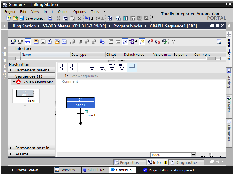
Пока
функциональный блок GRAPH_Sequence содержит
только один шаг. Теперь добавьте шаги
и переходы для процесса приготовления
и розлива сока. Для этого выделите
двойную стрелку шага и из контекстного
меню выполните команду Insert
element/Step and transition.
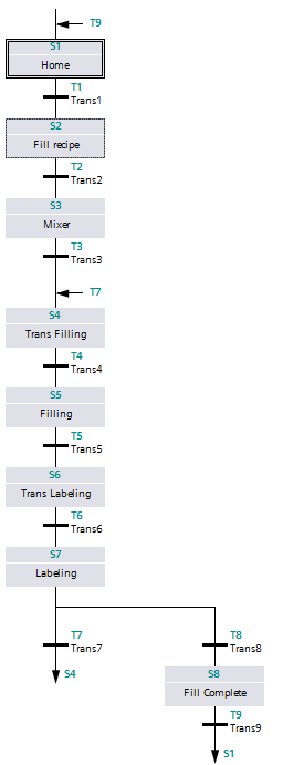
Как
видно, после шага 7 определено разветвление
потока выполнения. Для создания
разветвления выделите шаг S7 и из
контекстного меню выполните команду
Insert element/Open
Alternative branch.
После этого разместите шаг S8 – Fill
Complete.
Как
было указано выше, когда заполнено менее
10 бутылок, процесс заполнения бутылок
повторяется с шага S4
– Trans Filling.
Когда 10 бутылок заполнены, тогда
выполняется шаг S8
– Fill Complete и
далее происходит переход на начало
последовательности (шаг S1
Home) для
запуска процесса приготовления сока
по новой.
Для
вставки перехода выделите конец стрелки
после шага S7
– Labeling и из
контекстного меню выполните команду
Insert element/Jump.
При этом появляется список шагов.

Выберите
из этого списка шаг перехода S4
– Trans Filling.
При этом двойная стрелка преобразуется
на одинарную стрелку и рядом со стрелкой
появляется надпись S4. Также на верху
шага S4 появляется стрелка с надписью
Т7.
Аналогично
размещайте другой переход: после шага
S8
выполните переход на шаг S1
– Home.
14) Программирование действий шагов в редакторе Graph: квалификаторы действий n, r, s, l и события s0 и s1

Действия, которые
зависят от событий
Действия могут
быть логически скомбинированы с
событиями. Событие – это изменение
состояния шага или супервизора,
блокирование, квитирование, сообщение
или установка регистрации.
S1: Шаг активируется.
S0: Шаг деактивируется.
15) Программирование условий перехода на следующий шаг на примере индивидуального задания по срв. Создание разветвлений в программе Graph
Откройте
в редакторе программ шаг S1-Home.
Разместите нормально замкнутый контакт
в области T1–Trans1. Введите имя тега
Group_Fault
– тег, который предназначен для хранения
групповой ошибки. Пока этот тег не
определен. Для определения этого тега
из контекстного меню выполните команду
Define tag.
При этом появляется диалоговое окно
создания тега

В
этом окне определите тег со следующими
свойствами:
–
Адрес: M10.0
–
Тип данных: Bool
–
Таблица тегов:
Markers
Подтвердите
создание тега путем нажатия кнопки
Define.
Далее
скопируйте этот нормально замкнутый
контакт, откройте каждый шаг проекта и
скопированный замкнутый контакт вставьте
в область перехода каждого шага.
Параллельное
разветвление отвечает
обработке ветвей по логике И. Параллельное
разветвление начинается общим
переходом,
который активирует первый шаг во
всех параллельных
ветвях.
На рисунке 4.4 общими
переходами являются переходы Т3 и Т7.
Параллельное
разветвление заканчивается шагом,
подключенным к общему финальному
переходу. Финальный переход позволяет
следующий шаг только тогда, когда
выполнены все параллельные ветви.


Рисунок 4.3 —
Секвенсор с альтернативными ветвями
Рисунок 4.4 –
Секвенсор с параллельными ветвями
Постоянные
условия
Условия, которые
нужно выполнять в более чем одной точке
секвенсора, могут быть запрограммированы
как постоянные условия.
Для программирования
условий можно использовать элементы
контактной схемы – нормально разомкнутые
или нормально замкнутые контакты,
компараторы или элементы FBD. В постоянном
условии можно использовать до 32 элементов.
Результат вычисления
условий хранится элементом «катушка»
в LAD или блоком памяти в FBD.
Вызовы блока
Блоки, созданные
на других языках программирования,
могут быть вызванны с использованием
постоянных инструкций или действий в
FB S7-GRAPH. После того, как вызванный блок
будет выполнен, выполнение FB S7-GRAPH будет
продлено.
В S7-GRAPH можно вызвать
функции (FC) и функциональные блоки (FB),
запрограммированные на LAD, FBD, STL или SCL,
а также системные функции (SFC) и системные
функциональные блоки (SFB). Функциональным
блокам и системным функциональным
блокам должны быть назначены экземплярные
блоки данных DB. Имена блоков можно
использовать в абсолютном виде, например,
FC1 или символьно, например, Motor1. При
вызове блоков нужно обеспечить формальные
параметры вызываемого блока действительными
значениями.
16)
Программа вычисления срока годности
сока на языке SCL (на примере технологического
процесса приготовления сока). Поля типа
данных Date_And_Time. Перекрытие тега типа
Date_And_Time с массивом байтов/
Тип данных
Date_And_Time
содержит дату и время в BCD
формате в памяти длиной 8 байт. Например,
ниже указано хранение значения
2011-07-04-10:30:40.201 (July
4, 2011, 10:30, 40 seconds
201 milliseconds).
Последние 4 бита байта 7 хранят день
недели.

Перекрытие
тега типа Date_And_Time с массивом байтов
-
Для перекрытия предыдущего тега с
другим тегом, в разделе Temp
определите третий параметр со следующими
свойствами:
–
Имя: System_Time_Array
–
Тип данных: AT
После
ввода ключевого слова AT
автоматический создается составное
имя для нового тега, которое имеет
следующий формат:
<Имя нового тега>
AT
<Имя первого тега>
Тип
данных нового тега автоматически
определяется как Date_And_Time.
Измените этот тип на тип Array
[0 .. 7] of
Byte.
-
В разделе Temp
определите 4-й параметр со следующими
свойствами:
–
Имя: Year
–
Тип данных: Int
Этот
параметр предназначен для хранения
года, прочитанного из системного времени.
На
рисунке приведен вид интерфейсной части
этого программного блока.
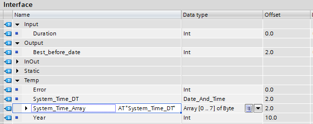
Интерфейсная
часть
блока
SCL_Best_before_date
-
Вычисление срока годности. Для определения
кода функционального блока на языке
SCL переходите в
область кода и наберите следующий код:
#Error
:= «RD_SYS_T» (OUT => #System_Time_DT);
#Year
:= BCD_TO_INT(#System_Time_Array[0]);
#Best_Before_Date
:= #Year + 2000 + #Duration;
Как
видно, в коде с помощью функции RD_SYS_T
считывается системное время и из него
выделяется год. Затем считывается срок
годности, путем сложения числа 2000 и
значения переменной #Duration.
Чертежно-графический редактор APM Graph. Руководство пользователя
Комментарии
Комментарии могут оставлять только зарегистрированные
участники
Авторизоваться
Порядок:
от старых к новым
Комментарии 1-1 из 1
Пельмень
, 13 марта 2009 в 22:51
#1
Ну как графический редактор не очень хорош, да и сложен в освоении, но как как одна из программ комплекса APM вполне заслуживает внимания
Порядок:
от старых к новым
graph(3)
2D graph for plotting X-Y coordinate data.
SYNOPSIS
graph pathName ?option value?…
DESCRIPTION
The graph command creates a graph for plotting
two-dimensional data (X-Y coordinates). It has many configurable
components: coordinate axes, elements, legend, grid lines, cross
hairs, etc. They allow you to customize the look and feel of the
graph.
INTRODUCTION
The graph command creates a new window for plotting
two-dimensional data (X-Y coordinates). Data points are plotted in a
rectangular area displayed in the center of the new window. This is the
plotting area. The coordinate axes are drawn in the
margins around the plotting area. By default, the legend is displayed
in the right margin. The title is displayed in top margin.
The graph widget is composed of several components: coordinate
axes, data elements, legend, grid, cross hairs, pens, postscript, and
annotation markers.
- axis
-
The graph has four standard axes (x, x2,
y, and y2), but you can create and display any number
of axes. Axes control what region of data is
displayed and how the data is scaled. Each axis consists of the axis
line, title, major and minor ticks, and tick labels. Tick labels
display the value at each major tick. - crosshairs
-
Cross hairs are used to position the mouse pointer relative to the X
and Y coordinate axes. Two perpendicular lines, intersecting at the
current location of the mouse, extend across the plotting area to the
coordinate axes. - element
-
An element represents a set of data points. Elements can be plotted
with a symbol at each data point and lines connecting the points.
The appearance of the element, such as its symbol, line width, and
color is configurable. - grid
-
Extends the major and minor ticks of the X-axis and/or Y-axis across the
plotting area. - legend
-
The legend displays the name and symbol of each data element.
The legend can be drawn in any margin or in the plotting area. - marker
-
Markers are used annotate or highlight areas of the graph. For
example, you could use a polygon marker to fill an area under a
curve, or a text marker to label a particular data point. Markers
come in various forms: text strings, bitmaps, connected line
segments, images, polygons, or embedded widgets. - pen
-
Pens define attributes (both symbol and line style) for elements.
Data elements use pens to specify how they should be drawn. A data
element may use many pens at once. Here, the particular pen
used for a data point is determined from each element’s weight
vector (see the element’s -weight and -style options). - postscript
-
The widget can generate encapsulated PostScript output. This component
has several options to configure how the PostScript is generated.
SYNTAX
-
graph pathName ?option value?...
The graph command creates a new window pathName and makes
it into a graph widget. At the time this command is invoked, there
must not exist a window named pathName, but pathName‘s
parent must exist. Additional options may be specified on the
command line or in the option database to configure aspects of the
graph such as its colors and font. See the configure operation
below for the exact details about what option and value
pairs are valid.
If successful, graph returns the path name of the widget. It
also creates a new Tcl command by the same name. You can use this
command to invoke various operations that query or modify the graph.
The general form is:
-
pathName operation ?arg?...
Both operation and its arguments determine the exact behavior of
the command. The operations available for the graph are described in
the
«GRAPH OPERATIONS»
section.
The command can also be used to access components of the graph.
-
pathName component operation ?arg?...
The operation, now located after the name of the component, is the
function to be performed on that component. Each component has its own
set of operations that manipulate that component. They will be
described below in their own sections.
EXAMPLE
The graph command creates a new graph.
-
# Create a new graph.  Plotting area is black.
graph .g -plotbackground black
A new Tcl command .g is also created. This command can be used
to query and modify the graph. For example, to change the title of
the graph to «My Plot», you use the new command and the graph’s
configure operation.
-
# Change the title.
.g configure -title "My Plot"
A graph has several components. To access a particular component you
use the component’s name. For example, to add data elements, you use
the new command and the element component.
-
# Create a new element named "line1"
.g element create line1 \
   -xdata { 0.2 0.4 0.6 0.8 1.0 1.2 1.4 1.6 1.8 2.0 } \
   -ydata { 26.18 50.46 72.85 93.31 111.86 128.47 143.14
     155.85 166.60 175.38 }
The element’s X-Y coordinates are specified using lists of
numbers. Alternately, BLT vectors could be used to hold the X-Y
coordinates.
-
# Create two vectors and add them to the graph.
vector xVec yVec
xVec set { 0.2 0.4 0.6 0.8 1.0 1.2 1.4 1.6 1.8 2.0 }
yVec set { 26.18 50.46 72.85 93.31 111.86 128.47 143.14 155.85
   166.60 175.38 }
.g element create line1 -xdata xVec -ydata yVec
The advantage of using vectors is that when you modify one, the graph
is automatically redrawn to reflect the new values.
-
# Change the y coordinate of the first point.
set yVector(0) 25.18
An element named e1 is now created in .b. It
is automatically added to the display list of elements. You can
use this list to control in what order elements are displayed.
To query or reset the element display list, you use the element’s
show operation.
-
# Get the current display list
set elemList [.b element show]
# Remove the first element so it won't be displayed.
.b element show [lrange $elemList 0 end]
The element will be displayed by as many bars as there are data points
(in this case there are ten). The bars will be drawn centered at the
x-coordinate of the data point. All the bars will have the same
attributes (colors, stipple, etc). The width of each bar is by
default one unit. You can change this with using the -barwidth
option.
-
# Change the X-Y coordinates of the first point.
set xVec(0) 0.18
set yVec(0) 25.18
An element named line1 is now created in .g. By
default, the element’s label in the legend will be also line1.
You can change the label, or specify no legend entry, again using the
element’s configure operation.
-
# Don't display "line1" in the legend.
.g element configure line1 -label ""
You can configure more than just the element’s label. An element has
many attributes such as symbol type and size, dashed or solid lines,
colors, line width, etc.
-
.g element configure line1 -symbol square -color red \
   -dashes { 2 4 2 } -linewidth 2 -pixels 2c
Four coordinate axes are automatically created: x, x2,
y, and y2. And by default, elements are mapped onto the
axes x and y. This can be changed with the -mapx
and -mapy options.
-
# Map "line1" on the alternate Y-axis "y2".
.g element configure line1 -mapy y2
Axes can be configured in many ways too. For example, you change the
scale of the Y-axis from linear to log using the axis component.
-
# Y-axis is log scale.
.g axis configure y -logscale yes
One important way axes are used is to zoom in on a particular data
region. Zooming is done by simply specifying new axis limits using
the -min and -max configuration options.
-
.g axis configure x -min 1.0 -max 1.5
.g axis configure y -min 12.0 -max 55.15
To zoom interactively, you link the axis configure operations with
some user interaction (such as pressing the mouse button), using the
bind command. To convert between screen and graph coordinates,
use the invtransform operation.
-
# Click the button to set a new minimum
bind .g <ButtonPress-1> {
    %W axis configure x -min [%W axis invtransform x %x]
    %W axis configure x -min [%W axis invtransform x %y]
}
By default, the limits of the axis are determined from data values.
To reset back to the default limits, set the -min and
-max options to the empty value.
-
# Reset the axes to autoscale again.
.g axis configure x -min {} -max {}
.g axis configure y -min {} -max {}
By default, the legend is drawn in the right margin. You can
change this or any legend configuration options using the
legend component.
-
# Configure the legend font, color, and relief
.g legend configure -position left -relief raised \
   -font fixed -fg blue
To prevent the legend from being displayed, turn on the -hide
option.
-
# Don't display the legend.
.g legend configure -hide yes
The graph widget has simple drawing procedures called markers.
They can be used to highlight or annotate data in the graph. The types
of markers available are bitmaps, images, polygons, lines, or windows.
Markers can be used, for example, to mark or brush points. In this
example, is a text marker that labels the data first point. Markers
are created using the marker component.
-
# Create a label for the first data point of "line1".
.g marker create text -name first_marker -coords { 0.2 26.18 } \
   -text "start" -anchor se -xoffset -10 -yoffset -10
This creates a text marker named first_marker. It will display
the text «start» near the coordinates of the first data point. The
-anchor, -xoffset, and -yoffset options are used
to display the marker above and to the left of the data point, so that
the data point isn’t covered by the marker. By default,
markers are drawn last, on top of data. You can change this with the
-under option.
-
# Draw the label before elements are drawn.
.g marker configure first_marker -under yes
You can add cross hairs or grid lines using the crosshairs and
grid components.
-
# Display both cross hairs and grid lines.
.g crosshairs configure -hide no -color red
.g grid configure -hide no -dashes { 2 2 }
# Set up a binding to reposition the crosshairs.
bind .g <Motion> {
    .g crosshairs configure -position @%x,%y
}
The crosshairs are repositioned as the mouse pointer is moved
in the graph. The pointer X-Y coordinates define the center
of the crosshairs.
Finally, to get hardcopy of the graph, use the postscript
component.
-
# Print the graph into file "file.ps"
.g postscript output file.ps -maxpect yes -decorations no
This generates a file file.ps containing the encapsulated
PostScript of the graph. The option -maxpect says to scale the
plot to the size of the page. Turning off the -decorations
option denotes that no borders or color backgrounds should be
drawn (i.e. the background of the margins, legend, and plotting
area will be white).
GRAPH OPERATIONS
- pathName axis operation ?arg?…
-
See the
«AXIS COMPONENTS»
section. - pathName bar elemName ?option value?…
-
Creates a new barchart element elemName. It’s an
error if an element elemName already exists.
See the manual for barchart for details about
what option and value pairs are valid. - pathName cget option
-
Returns the current value of the configuration option given by
option. Option may be any option described
below for the configure operation. - pathName configure ?option value?…
-
Queries or modifies the configuration options of the graph. If
option isn’t specified, a list describing the current
options for pathName is returned. If option is specified,
but not value, then a list describing option is returned.
If one or more option and value pairs are specified, then
for each pair, the option option is set to value.
The following options are valid.-
- -aspect width/height
- Force a fixed aspect ratio of width/height, a floating point number.
- -background color
-
Sets the background color. This includes the margins and
legend, but not the plotting area. - -borderwidth pixels
-
Sets the width of the 3-D border around the outside edge of the widget. The
-relief option determines if the border is to be drawn. The
default is 2. - -bottommargin pixels
-
If non-zero, overrides the computed size of the margin extending
below the X-coordinate axis.
If pixels is 0, the automatically computed size is used.
The default is 0. - -bufferelements boolean
-
Indicates whether an internal pixmap to buffer the display of data
elements should be used. If boolean is true, data elements are
drawn to an internal pixmap. This option is especially useful when
the graph is redrawn frequently while the remains data unchanged (for
example, moving a marker across the plot). See the
«SPEED TIPS»
section.
The default is 1. - -cursor cursor
- Specifies the widget’s cursor. The default cursor is crosshair.
- -font fontName
-
Specifies the font of the graph title. The default is
*-Helvetica-Bold-R-Normal-*-18-180-*. - -halo pixels
-
Specifies a maximum distance to consider when searching for the
closest data point (see the element’s closest operation below).
Data points further than pixels away are ignored. The default is
0.5i. - -height pixels
-
Specifies the requested height of widget. The default is
4i. - -invertxy boolean
-
Indicates whether the placement X-axis and Y-axis should be inverted. If
boolean is true, the X and Y axes are swapped. The default is
0. - -justify justify
-
Specifies how the title should be justified. This matters only when
the title contains more than one line of text. Justify must be
left, right, or center. The default is
center. - -leftmargin pixels
-
If non-zero, overrides the computed size of the margin extending
from the left edge of the window to the Y-coordinate axis.
If pixels is 0, the automatically computed size is used.
The default is 0. - -plotbackground color
-
Specifies the background color of the plotting area. The default is
white. - -plotborderwidth pixels
-
Sets the width of the 3-D border around the plotting area. The
-plotrelief option determines if a border is drawn. The
default is 2. - -plotpadx pad
-
Sets the amount of padding to be added to the left and right sides of
the plotting area. Pad can be a list of one or two screen
distances. If pad has two elements, the left side of the
plotting area entry is padded by the first distance and the right side
by the second. If pad is just one distance, both the left and
right sides are padded evenly. The default is 8. - -plotpady pad
-
Sets the amount of padding to be added to the top and bottom of the
plotting area. Pad can be a list of one or two screen
distances. If pad has two elements, the top of the plotting
area is padded by the first distance and the bottom by the second. If
pad is just one distance, both the top and bottom are padded
evenly. The default is 8. - -plotrelief relief
-
Specifies the 3-D effect for the plotting area. Relief
specifies how the interior of the plotting area should appear relative
to rest of the graph; for example, raised means the plot should
appear to protrude from the graph, relative to the surface of the
graph. The default is sunken. - -relief relief
-
Specifies the 3-D effect for the graph widget. Relief
specifies how the graph should appear relative to widget it is packed
into; for example, raised means the graph should
appear to protrude. The default is flat. - -rightmargin pixels
-
If non-zero, overrides the computed size of the margin extending
from the plotting area to the right edge of
the window. By default, the legend is drawn in this margin.
If pixels is 0, the automatically computed size is used.
The default is 0. - -takefocus focus
-
Provides information used when moving the focus from window to window
via keyboard traversal (e.g., Tab and Shift-Tab). If focus is
0, this means that this window should be skipped entirely during
keyboard traversal. 1 means that the this window should always
receive the input focus. An empty value means that the traversal
scripts make the decision whether to focus on the window.
The default is «». - -tile image
-
Specifies a tiled background for the widget. If image isn’t
«», the background is tiled using image.
Otherwise, the normal background color is drawn (see the
-background option). Image must be an image created
using the Tk image command. The default is «». - -title text
-
Sets the title to text. If text is «»,
no title will be displayed. - -topmargin pixels
-
If non-zero, overrides the computed size of the margin above the x2
axis. If pixels is 0, the automatically computed size
is used. The default is 0. - -width pixels
-
Specifies the requested width of the widget. The default is
5i.
-
- pathName crosshairs operation ?arg?
-
See the
«CROSSHAIRS COMPONENT»
section. - pathName element operation ?arg?…
-
See the
«ELEMENT COMPONENTS»
section. - pathName extents item
-
Returns the size of a particular item in the graph. Item must
be either leftmargin, rightmargin, topmargin,
bottommargin, plotwidth, or plotheight. - pathName grid operation ?arg?…
-
See the
«GRID COMPONENT»
section. - pathName invtransform winX winY
-
Performs an inverse coordinate transformation, mapping window
coordinates back to graph coordinates, using the standard X-axis and Y-axis.
Returns a list of containing the X-Y graph coordinates. - pathName inside x y
-
Returns 1 is the designated screen coordinate (x and y)
is inside the plotting area and 0 otherwise. - pathName legend operation ?arg?…
-
See the
«LEGEND COMPONENT»
section. - pathName line operation arg…
- The operation is the same as element.
- pathName marker operation ?arg?…
-
See the
«MARKER COMPONENTS»
section. - pathName postscript operation ?arg?…
-
See the
«POSTSCRIPT COMPONENT»
section. - pathName snap ?switches? outputName
-
Takes a snapshot of the graph, saving the output in outputName.
The following switches are available.-
- -format format
-
Specifies how the snapshot is output. Format may be one of
the following listed below. The default is photo.-
- photo
-
Saves a Tk photo image. OutputName represents the name of a
Tk photo image that must already have been created. - wmf
-
Saves an Aldus Placeable Metafile. OutputName represents the
filename where the metafile is written. If outputName is
CLIPBOARD, then output is written directly to the Windows
clipboard. This format is available only under Microsoft Windows. - emf
-
Saves an Enhanced Metafile. OutputName represents the filename
where the metafile is written. If outputName is
CLIPBOARD, then output is written directly to the Windows
clipboard. This format is available only under Microsoft Windows.
-
- -height size
-
Specifies the height of the graph. Size is a screen distance.
The graph will be redrawn using this dimension, rather than its
current window height. - -width size
-
Specifies the width of the graph. Size is a screen distance.
The graph will be redrawn using this dimension, rather than its
current window width.
-
- pathName transform x y
-
Performs a coordinate transformation, mapping graph coordinates to
window coordinates, using the standard X-axis and Y-axis.
Returns a list containing the X-Y screen coordinates. - pathName xaxis operation ?arg?…
- pathName x2axis operation ?arg?…
- pathName yaxis operation ?arg?…
- pathName y2axis operation ?arg?…
-
See the
«AXIS COMPONENTS»
section.
GRAPH COMPONENTS
A graph is composed of several components: coordinate axes, data
elements, legend, grid, cross hairs, postscript, and annotation
markers. Instead of one big set of configuration options and
operations, the graph is partitioned, where each component has its own
configuration options and operations that specifically control that
aspect or part of the graph.
AXIS COMPONENTS
Four coordinate axes are automatically created: two X-coordinate axes
(x and x2) and two Y-coordinate axes (y, and
y2). By default, the axis x is located in the bottom
margin, y in the left margin, x2 in the top margin, and
y2 in the right margin.
An axis consists of the axis line, title, major and minor ticks, and
tick labels. Major ticks are drawn at uniform intervals along the
axis. Each tick is labeled with its coordinate value. Minor ticks
are drawn at uniform intervals within major ticks.
The range of the axis controls what region of data is plotted.
Data points outside the minimum and maximum limits of the axis are
not plotted. By default, the minimum and maximum limits are
determined from the data, but you can reset either limit.
You can have several axes. To create an axis, invoke
the axis component and its create operation.
-
# Create a new axis called "tempAxis"
.g axis create tempAxis
You map data elements to an axis using the element’s -mapy and -mapx
configuration options. They specify the coordinate axes an element
is mapped onto.
-
# Now map the tempAxis data to this axis.
.g element create "e1" -xdata $x -ydata $y -mapy tempAxis
Any number of axes can be displayed simultaneously. They are drawn in
the margins surrounding the plotting area. The default axes x
and y are drawn in the bottom and left margins. The axes
x2 and y2 are drawn in top and right margins. By
default, only x and y are shown. Note that the axes
can have different scales.
To display a different axis or more than one axis, you invoke one of
the following components: xaxis, yaxis, x2axis, and
y2axis. Each component has a use operation that
designates the axis (or axes) to be drawn in that corresponding
margin: xaxis in the bottom, yaxis in the left,
x2axis in the top, and y2axis in the right.
-
# Display the axis tempAxis in the left margin.
.g yaxis use tempAxis
The use operation takes a list of axis names as its last
argument. This is the list of axes to be drawn in this margin.
You can configure axes in many ways. The axis scale can be linear or
logarithmic. The values along the axis can either monotonically
increase or decrease. If you need custom tick labels, you can specify
a Tcl procedure to format the label any way you wish. You can control
how ticks are drawn, by changing the major tick interval or the number
of minor ticks. You can define non-uniform tick intervals, such as
for time-series plots.
- pathName axis bind tagName ?sequence? ?command?
-
Associates command with tagName such that whenever the
event sequence given by sequence occurs for an axis with this
tag, command will be invoked. The syntax is similar to the
bind command except that it operates on graph axes, rather
than widgets. See the bind manual entry for
complete details on sequence and the substitutions performed on
command before invoking it.If all arguments are specified then a new binding is created, replacing
any existing binding for the same sequence and tagName.
If the first character of command is + then command
augments an existing binding rather than replacing it.
If no command argument is provided then the command currently
associated with tagName and sequence (it’s an error occurs
if there’s no such binding) is returned. If both command and
sequence are missing then a list of all the event sequences for
which bindings have been defined for tagName. - pathName axis cget axisName option
-
Returns the current value of the option given by option for
axisName. Option may be any option described below
for the axis configure operation. - pathName axis configure axisName ?axisName?… ?option value?…
-
Queries or modifies the configuration options of axisName.
Several axes can be changed. If option isn’t specified, a list
describing all the current options for axisName is returned. If
option is specified, but not value, then a list describing
option is returned. If one or more option and value
pairs are specified, then for each pair, the axis option option
is set to value. The following options are valid for axes.-
- -bindtags tagList
-
Specifies the binding tags for the axis. TagList is a list
of binding tag names. The tags and their order will determine how
events for axes are handled. Each tag in the list matching the current event
sequence will have its Tcl command executed. Implicitly the name of
the element is always the first tag in the list. The default value is
all. - -color color
-
Sets the color of the axis and tick labels.
The default is black. - -command prefix
-
Specifies a Tcl command to be invoked when formatting the axis tick
labels. Prefix is a string containing the name of a Tcl proc and
any extra arguments for the procedure. This command is invoked for each
major tick on the axis. Two additional arguments are passed to the
procedure: the pathname of the widget and the current the numeric
value of the tick. The procedure returns the formatted tick label. If
«» is returned, no label will appear next to the tick. You can
get the standard tick labels again by setting prefix to
«». The default is «».Please note that this procedure is invoked while the graph is redrawn.
You may query configuration options. But do not them, because this
can have unexpected results. - -descending boolean
-
Indicates whether the values along the axis are monotonically increasing or
decreasing. If boolean is true, the axis values will be
decreasing. The default is 0. - -hide boolean
-
Indicates if the axis is displayed. If boolean is false the axis
will be displayed. Any element mapped to the axis is displayed regardless.
The default value is 0. - -justify justify
-
Specifies how the axis title should be justified. This matters only
when the axis title contains more than one line of text. Justify
must be left, right, or center. The default is
center. - -limits formatStr
-
Specifies a printf-like description to format the minimum and maximum
limits of the axis. The limits are displayed at the top/bottom or
left/right sides of the plotting area. FormatStr is a list of
one or two format descriptions. If one description is supplied, both
the minimum and maximum limits are formatted in the same way. If two,
the first designates the format for the minimum limit, the second for
the maximum. If «» is given as either description, then
the that limit will not be displayed. The default is «». - -linewidth pixels
-
Sets the width of the axis and tick lines. The default is 1
pixel. - -logscale boolean
-
Indicates whether the scale of the axis is logarithmic or linear. If
boolean is true, the axis is logarithmic. The default scale is
linear. - -loose boolean
-
Indicates whether the limits of the axis should fit the data points tightly,
at the outermost data points, or loosely, at the outer tick intervals.
If the axis limit is set with the -min or -max option, the axes are
displayed tightly.
If boolean is true, the axis range is «loose».
The default is 0. - -majorticks majorList
-
Specifies where to display major axis ticks. You can use this option
to display ticks at non-uniform intervals. MajorList is a list
of axis coordinates designating the location of major ticks. No
minor ticks are drawn. If majorList is «»,
major ticks will be automatically computed. The default is «». - -max value
-
Sets the maximum limit of axisName. Any data point greater
than value is not displayed. If value is «»,
the maximum limit is calculated using the largest data value.
The default is «». - -min value
-
Sets the minimum limit of axisName. Any data point less than
value is not displayed. If value is «»,
the minimum limit is calculated using the smallest data value.
The default is «». - -minorticks minorList
-
Specifies where to display minor axis ticks. You can use this option
to display minor ticks at non-uniform intervals. MinorList is a
list of real values, ranging from 0.0 to 1.0, designating the placement of
a minor tick. No minor ticks are drawn if the -majortick
option is also set. If minorList is «», minor ticks will
be automatically computed. The default is «». - -rotate theta
-
Specifies the how many degrees to rotate the axis tick labels.
Theta is a real value representing the number of degrees
to rotate the tick labels. The default is 0.0 degrees. - -scrollcommand command
-
Specify the prefix for a command used to communicate with scrollbars
for this axis, such as .sbar set. - -scrollmax value
-
Sets the maximum limit of the axis scroll region. If value is
«», the maximum limit is calculated using the largest data
value. The default is «». - -scrollmin value
-
Sets the minimum limit of axis scroll region. If value is
«», the minimum limit is calculated using the smallest data
value. The default is «». - -showticks boolean
-
Indicates whether axis ticks should be drawn. If boolean is
true, ticks are drawn. If false, only the
axis line is drawn. The default is 1. - -stepsize value
-
Specifies the interval between major axis ticks. If value isn’t
a valid interval (must be less than the axis range),
the request is ignored and the step size is automatically calculated. - -subdivisions number
-
Indicates how many minor axis ticks are
to be drawn. For example, if number is two, only one minor
tick is drawn. If number is one, no minor ticks are
displayed. The default is 2. - -tickfont fontName
-
Specifies the font for axis tick labels. The default is
*-Courier-Bold-R-Normal-*-100-*. - -ticklength pixels
-
Sets the length of major and minor ticks (minor ticks are half the
length of major ticks). If pixels is less than zero, the axis
will be inverted with ticks drawn pointing towards the plot. The
default is 0.1i. - -title text
-
Sets the title of the axis. If text is
«», no axis title will be displayed. - -titlealternate boolean
-
Indicates to display the axis title in its alternate location.
Normally the axis title is centered along the axis. This option
places the axis either to the right (horizontal axes) or above
(vertical axes) the axis. The default is 0. - -titlecolor color
- Sets the color of the axis title. The default is black.
- -titlefont fontName
-
Specifies the font for axis title. The default is
*-Helvetica-Bold-R-Normal-*-14-140-*.
Axis configuration options may be also be set by the option
command. The resource class is Axis. The resource names
are the names of the axes (such as x or x2).-
option add *Graph.Axis.Color  blue
option add *Graph.x.LogScale  true
option add *Graph.x2.LogScale false
-
- pathName axis create axisName ?option value?…
-
Creates a new axis by the name axisName. No axis by the same
name can already exist. Option and value are described
in above in the axis configure operation. - pathName axis delete ?axisName?…
-
Deletes the named axes. An axis is not really
deleted until it is not longer in use, so it’s safe to delete
axes mapped to elements. - pathName axis invtransform axisName value
-
Performs the inverse transformation, changing the screen coordinate
value to a graph coordinate, mapping the value mapped to
axisName. Returns the graph coordinate. - pathName axis limits axisName
-
Returns a list of the minimum and maximum limits for axisName. The order
of the list is min max. - pathName axis names ?pattern?…
-
Returns a list of axes matching zero or more patterns. If no
pattern argument is give, the names of all axes are returned. - pathName axis transform axisName value
-
Transforms the coordinate value to a screen coordinate by mapping
the it to axisName. Returns the transformed screen coordinate. - pathName axis view axisName
- Change the viewable area of this axis. Use as an argument to a scrollbar’s «-command«.
The default axes are x, y, x2, and y2.
But you can display more than four axes simultaneously. You can also
swap in a different axis with use operation of the special axis
components: xaxis, x2axis, yaxis, and y2axis.
-
.g create axis temp
.g create axis time
...
.g xaxis use temp
.g yaxis use time
Only the axes specified for use are displayed on the screen.
The xaxis, x2axis, yaxis, and y2axis
components operate on an axis location rather than a specific axis
like the more general axis component does. They implicitly
control the axis that is currently using to that location. By
default, xaxis uses the x axis, yaxis uses
y, x2axis uses x2, and y2axis uses
y2. When more than one axis is displayed in a margin, it
represents the first axis displayed.
The following operations are available for axes. They mirror exactly
the operations of the axis component. The axis argument
must be xaxis, x2axis, yaxis, or y2axis. This
feature is deprecated since more than one axis can now be used a
margin. You should only use the xaxis, x2axis,
yaxis, and y2axis components with the use operation.
For all other operations, use the general axis component
instead.
- pathName axis cget option
- pathName axis configure ?option value?…
- pathName axis invtransform value
- pathName axis limits
- pathName axis transform value
- pathName axis use ?axisName?
-
Designates the axis axisName is to be displayed at this
location. AxisName can not be already in use at another location.
This command returns the name of the axis currently using this location.
CROSSHAIRS COMPONENT
Cross hairs consist of two intersecting lines (one vertical and one horizontal)
drawn completely across the plotting area. They are used to position
the mouse in relation to the coordinate axes. Cross hairs differ from line
markers in that they are implemented using XOR drawing primitives.
This means that they can be quickly drawn and erased without redrawing
the entire graph. Note that crosshair are enabled by calling
Blt_Crosshairs and turned off by calling Blt_ResetCrosshairs.
Similarly call Blt_ZoomStack for zooming.
The following operations are available for cross hairs:
- pathName crosshairs cget option
-
Returns the current value of the cross hairs configuration option
given by option. Option may be any option
described below for the cross hairs configure operation. - pathName crosshairs configure ?option value?…
-
Queries or modifies the configuration options of the cross hairs. If
option isn’t specified, a list describing all the current
options for the cross hairs is returned. If option is specified,
but not value, then a list describing option is returned.
If one or more option and value pairs are specified, then
for each pair, the cross hairs option option is set to
value.
The following options are available for cross hairs.-
- -color color
- Sets the color of the cross hairs. The default is black.
- -dashes dashList
-
Sets the dash style of the cross hairs. DashList is a list of up
to 11 numbers that alternately represent the lengths of the dashes
and gaps on the cross hair lines. Each number must be between 1 and
255. If dashList is «», the cross hairs will be solid
lines. - -hide boolean
-
Indicates whether cross hairs are drawn. If boolean is true,
cross hairs are not drawn. The default is yes. - -linewidth pixels
- Set the width of the cross hair lines. The default is 1.
- -position pos
-
Specifies the screen position where the cross hairs intersect.
Pos must be in the form «@x,y«, where x and y
are the window coordinates of the intersection.
Cross hairs configuration options may be also be set by the
option command. The resource name and class are
crosshairs and Crosshairs respectively.-
option add *Graph.Crosshairs.LineWidth 2
option add *Graph.Crosshairs.Color     red
-
- pathName crosshairs off
- Turns off the cross hairs.
- pathName crosshairs on
- Turns on the display of the cross hairs.
- pathName crosshairs toggle
-
Toggles the current state of the cross hairs, alternately mapping and
unmapping the cross hairs.
ELEMENT COMPONENTS
A data element represents a set of data. It contains x and y vectors
containing the coordinates of the data points. Elements can be
displayed with a symbol at each data point and lines connecting the
points. Elements also control the appearance of the data, such as the
symbol type, line width, color etc.
When new data elements are created, they are automatically added to a
list of displayed elements. The display list controls what elements
are drawn and in what order.
The following operations are available for elements.
- pathName element activate elemName ?index?…
-
Specifies the data points of element elemName to be drawn
using active foreground and background colors. ElemName is the
name of the element and index is a number representing the index
of the data point. If no indices are present then all data points
become active. - pathName element bind tagName ?sequence? ?command?
-
Associates command with tagName such that whenever the
event sequence given by sequence occurs for an element with this
tag, command will be invoked. The syntax is similar to the
bind command except that it operates on graph elements, rather
than widgets. See the bind manual entry for
complete details on sequence and the substitutions performed on
command before invoking it.If all arguments are specified then a new binding is created, replacing
any existing binding for the same sequence and tagName.
If the first character of command is + then command
augments an existing binding rather than replacing it.
If no command argument is provided then the command currently
associated with tagName and sequence (it’s an error occurs
if there’s no such binding) is returned. If both command and
sequence are missing then a list of all the event sequences for
which bindings have been defined for tagName. - pathName element cget elemName option
-
Returns the current value of the element configuration option given by
option. Option may be any of the options described below
for the element configure operation. - pathName element closest x y varName ?option value?… ?elemName?…
-
Searches for the data point closest to the window coordinates x
and y. By default, all elements are searched. Hidden elements
(see the -hide option is false) are ignored. You can limit the
search by specifying only the elements you want to be considered.
ElemName must be the name of an element that is not be hidden.
VarName is the name of a Tcl array variable and will contain
the search results: the name of the closest element, the index of
the closest data point, and the graph coordinates of the point. Returns
0, if no data point within the threshold distance can be found,
otherwise 1 is returned. The following
option—value pairs are available.-
- -along direction
-
Search for the closest element using the following criteria:
-
- x
- Find closest element vertically from the given X-coordinate.
- y
- Find the closest element horizontally from the given Y-coordinate.
- both
-
Find the closest element for the given point (using both the X and Y
coordinates).
-
- -halo pixels
-
Specifies a threshold distance where selected data points are ignored.
Pixels is a valid screen distance, such as 2 or 1.2i.
If this option isn’t specified, then it defaults to the value of the
graph’s -halo option. - -interpolate string
-
Indicates whether to consider projections that lie along the line segments
connecting data points when searching for the closest point.
The default value is 0. The values for string are
described below.-
- no
- Search only for the closest data point.
- yes
-
Search includes projections that lie along the
line segments connecting the data points.
-
-
- pathName element configure elemName ?elemName… ?option value?…
-
Queries or modifies the configuration options for elements. Several
elements can be modified at the same time. If option isn’t
specified, a list describing all the current options for
elemName is returned. If option is specified, but not
value, then a list describing the option option is
returned. If one or more option and value pairs are
specified, then for each pair, the element option option is set
to value. The following options are valid for elements.-
- -activepen penName
-
Specifies pen to use to draw active element. If penName is
«», no active elements will be drawn. The default is
activeLine. - -bindtags tagList
-
Specifies the binding tags for the element. TagList is a list
of binding tag names. The tags and their order will determine how
events are handled for elements. Each tag in the list matching the
current event
sequence will have its Tcl command executed. Implicitly the name of
the element is always the first tag in the list. The default value is
all. - -color color
- Sets the color of the traces connecting the data points.
- -dashes dashList
-
Sets the dash style of element line. DashList is a list of up to
11 numbers that alternately represent the lengths of the dashes and
gaps on the element line. Each number must be between 1 and 255. If
dashList is «», the lines will be solid. - -data coordList
-
Specifies the X-Y coordinates of the data. CoordList is a
list of numeric expressions representing the X-Y coordinate pairs
of each data point. - -fill color
-
Sets the interior color of symbols. If color is «», then
the interior of the symbol is transparent. If color is
defcolor, then the color will be the same as the -color
option. The default is defcolor. - -hide boolean
-
Indicates whether the element is displayed.
The default is no. - -label text
-
Sets the element’s label in the legend. If text
is «», the element will have no entry in the legend.
The default label is the element’s name. - -linewidth pixels
-
Sets the width of the connecting lines between data points. If
pixels is 0, no connecting lines will be drawn between
symbols. The default is 0. - -mapx xAxis
-
Selects the X-axis to map the element’s X-coordinates onto.
XAxis must be the name of an axis. The default is x. - -mapy yAxis
-
Selects the Y-axis to map the element’s Y-coordinates onto.
YAxis must be the name of an axis. The default is y. - -offdash color
-
Sets the color of the stripes when traces are dashed (see the
-dashes option). If color is «», then the «off»
pixels will represent gaps instead of stripes. If color is
defcolor, then the color will be the same as the -color
option. The default is defcolor. - -outline color
-
Sets the color or the outline around each symbol. If color is
«», then no outline is drawn. If color is defcolor,
then the color will be the same as the -color option. The
default is defcolor. - -pen penname
- Set the pen to use for this element.
- -outlinewidth pixels
-
Sets the width of the outline bordering each symbol. If pixels
is 0, no outline will be drawn. The default is 1. - -pixels pixels
-
Sets the size of symbols. If pixels is 0, no symbols will
be drawn. The default is 0.125i. - -scalesymbols boolean
-
If boolean is true, the size of the symbols
drawn for elemName will change with scale of the X-axis and Y-axis.
At the time this option is set, the current ranges of the axes are
saved as the normalized scales (i.e scale factor is 1.0) and the
element is drawn at its designated size (see the -pixels
option). As the scale of the axes change, the symbol will be scaled
according to the smaller of the X-axis and Y-axis scales. If boolean
is false, the element’s symbols are drawn at the designated size,
regardless of axis scales. The default is 0. - -smooth smooth
-
Specifies how connecting line segments are drawn between data points.
Smooth can be either linear, step, natural, or
quadratic. If smooth is linear, a single line
segment is drawn, connecting both data points. When smooth is
step, two line segments are drawn. The first is a horizontal
line segment that steps the next X-coordinate. The second is a
vertical line, moving to the next Y-coordinate. Both natural and
quadratic generate multiple segments between data points. If
natural, the segments are generated using a cubic spline. If
quadratic, a quadratic spline is used. The default is
linear. - -styles styleList
-
Specifies what pen to use based on the range of weights given.
StyleList is a list of style specifications. Each style
specification, in turn, is a list consisting of a pen name, and
optionally a minimum and maximum range. Data points whose weight (see
the -weight option) falls in this range, are drawn with this
pen. If no range is specified it defaults to the index of the pen in
the list. Note that this affects only symbol attributes. Line
attributes, such as line width, dashes, etc. are ignored. - -symbol symbol
-
Specifies the symbol for data points. Symbol can be either
square, circle, diamond, plus, cross,
splus, scross, triangle, «» (where no symbol
is drawn), or a bitmap. Bitmaps are specified as «source
?mask?», where source is the name of the bitmap, and
mask is the bitmap’s optional mask. The default is
circle. - -trace direction
-
Indicates whether connecting lines between data points (whose
X-coordinate values are either increasing or decreasing) are drawn.
Direction
must be increasing, decreasing, or both. For
example, if direction is increasing, connecting lines will
be drawn only between those data points where X-coordinate values are
monotonically increasing. If direction is both,
connecting lines will be draw between all data points. The default is
both. - -weights wVec
-
Specifies the weights of the individual data points. This,
with the list pen styles (see the -styles option),
controls how data points are drawn. WVec is the name of a BLT
vector or a list of numeric expressions representing the weights for
each data point. - -xdata xVec
-
Specifies the X-coordinates of the data. XVec is the name of
a BLT vector or a list of numeric expressions. - -ydata yVec
-
Specifies the Y-coordinates of the data. YVec is the name of
a BLT vector or a list of numeric expressions.
Element configuration options may also be set by the option
command. The resource class is Element. The resource name is
the name of the element.-
option add *Graph.Element.symbol line
option add *Graph.e1.symbol line
-
- pathName element create elemName ?option value?…
-
Creates a new element elemName. It’s an error is
an element elemName already exists. If
additional arguments are present, they specify options valid for
the element configure operation. - pathName element deactivate elemName ?elemName?…
-
Deactivates all the elements matching pattern.
Elements whose names match any of the patterns given are redrawn using
their normal colors. - pathName element delete ?elemName?…
- Deletes all the named elements. The graph is automatically redrawn.
- pathName element exists elemName
-
Returns 1 if an element elemName currently exists and
0 otherwise. - pathName element names ?pattern?…
-
Returns the elements matching one or more pattern. If no
pattern is given, the names of all elements is returned. - pathName element show ?nameList?
-
Queries or modifies the element display list. The element display
list designates the elements drawn and in what
order. NameList is a list of elements to be displayed in the
order they are named. If there is no nameList argument,
the current display list is returned. - pathName element type elemName
-
Returns the type of elemName.
If the element is a bar element, the commands returns the string
«bar», otherwise it returns «line».
GRID COMPONENT
Grid lines extend from the major and minor ticks of each axis
horizontally or vertically across the plotting area. The following
operations are available for grid lines.
- pathName grid cget option
-
Returns the current value of the grid line configuration option given by
option. Option may be any option described below
for the grid configure operation. - pathName grid configure ?option value?…
-
Queries or modifies the configuration options for grid lines. If
option isn’t specified, a list describing all the current
grid options for pathName is returned. If option is specified,
but not value, then a list describing option is
returned. If one or more option and value pairs are
specified, then for each pair, the grid line option option is set to
value. The following options are valid for grid lines.-
- -color color
- Sets the color of the grid lines. The default is black.
- -dashes dashList
-
Sets the dash style of the grid lines. DashList is a list of up
to 11 numbers that alternately represent the lengths of the dashes
and gaps on the grid lines. Each number must be between 1 and 255.
If dashList is «», the grid will be solid lines. - -hide boolean
-
Indicates whether the grid should be drawn. If boolean
is true, grid lines are not shown. The default is yes. - -linewidth pixels
- Sets the width of grid lines. The default width is 1.
- -mapx xAxis
-
Specifies the X-axis to display grid lines. XAxis
must be the name of an axis or «» for no grid lines.
The default is «». - -mapy yAxis
-
Specifies the Y-axis to display grid lines. YAxis
must be the name of an axis or «» for no grid lines.
The default is y. - -minor boolean
-
Indicates whether the grid lines should be drawn for minor ticks.
If boolean is true, the lines will appear at
minor tick intervals. The default is 1.
Grid configuration options may also be set by the
option command. The resource name and class are grid and
Grid respectively.-
option add *Graph.grid.LineWidth 2
option add *Graph.Grid.Color     black
- -raised boolean
- Grid is to be raised or drawn over elements.
-
- pathName grid off
- Turns off the display the grid lines.
- pathName grid on
- Turns on the display the grid lines.
- pathName grid toggle
- Toggles the display of the grid.
LEGEND COMPONENT
The legend displays a list of the data elements. Each entry consists
of the element’s symbol and label. The legend can appear in any
margin (the default location is in the right margin). It
can also be positioned anywhere within the plotting area.
The following operations are valid for the legend.
- pathName legend activate pattern…
-
Selects legend entries to be drawn using the active legend colors and relief.
All entries whose element names match pattern are selected. To
be selected, the element name must match only one pattern. - pathName legend bind tagName ?sequence? ?command?
-
Associates command with tagName such that whenever the
event sequence given by sequence occurs for a legend entry with this
tag, command will be invoked. Implicitly the element names
in the entry are tags. The syntax is similar to the
bind command except that it operates on legend entries, rather
than widgets. See the bind manual entry for
complete details on sequence and the substitutions performed on
command before invoking it.If all arguments are specified then a new binding is created, replacing
any existing binding for the same sequence and tagName.
If the first character of command is + then command
augments an existing binding rather than replacing it.
If no command argument is provided then the command currently
associated with tagName and sequence (it’s an error occurs
if there’s no such binding) is returned. If both command and
sequence are missing then a list of all the event sequences for
which bindings have been defined for tagName. - pathName legend cget option
-
Returns the current value of a legend configuration option.
Option may be any option described below in the
legend configure operation. - pathName legend configure ?option value?…
-
Queries or modifies the configuration options for the legend. If
option isn’t specified, a list describing the current
legend options for pathName is returned. If option is
specified, but not value, then a list describing option is
returned. If one or more option and value pairs are
specified, then for each pair, the legend option option is set
to value. The following options are valid for the legend.-
- -activebackground color
-
Sets the background color for active legend entries. All legend
entries marked active (see the legend activate operation) are
drawn using this background color. - -activeborderwidth pixels
-
Sets the width of the 3-D border around the outside edge of the active legend
entries. The default is 2. - -activeforeground color
-
Sets the foreground color for active legend entries. All legend
entries marked as active (see the legend activate operation) are
drawn using this foreground color. - -activerelief relief
-
Specifies the 3-D effect desired for active legend entries.
Relief denotes how the interior of the entry should appear
relative to the legend; for example, raised means the entry
should appear to protrude from the legend, relative to the surface of
the legend. The default is flat. - -anchor anchor
-
Tells how to position the legend relative to the positioning point for
the legend. This is dependent on the value of the -position
option. The default is center.-
- left or right
- The anchor describes how to position the legend vertically.
- top or bottom
- The anchor describes how to position the legend horizontally.
- @x,y
-
The anchor specifies how to position the legend relative to the
positioning point. For example, if anchor is center then
the legend is centered on the point; if anchor is n then
the legend will be drawn such that the top center point of the
rectangular region occupied by the legend will be at the positioning
point. - plotarea
-
The anchor specifies how to position the legend relative to the
plotting area. For example, if anchor is center then the
legend is centered in the plotting area; if anchor is ne
then the legend will be drawn such that occupies the upper right
corner of the plotting area.
-
- -background color
-
Sets the background color of the legend. If color is «»,
the legend background with be transparent. - -bindtags tagList
-
Specifies the binding tags for legend entries. TagList is a list
of binding tag names. The tags and their order will determine how
events are handled for legend entries. Each tag in the list matching
the current event sequence will have its Tcl command executed. The
default value is all. - -borderwidth pixels
-
Sets the width of the 3-D border around the outside edge of the legend (if
such border is being drawn; the relief option determines this).
The default is 2 pixels. - -font fontName
-
FontName specifies a font to use when drawing the labels of each
element into the legend. The default is
*-Helvetica-Bold-R-Normal-*-12-120-*. - -foreground color
-
Sets the foreground color of the text drawn for the element’s label.
The default is black. - -hide boolean
-
Indicates whether the legend should be displayed. If boolean is
true, the legend will not be draw. The default is no. - -ipadx pad
-
Sets the amount of internal padding to be added to the width of each
legend entry. Pad can be a list of one or two screen distances. If
pad has two elements, the left side of the legend entry is
padded by the first distance and the right side by the second. If
pad is just one distance, both the left and right sides are padded
evenly. The default is 2. - -ipady pad
-
Sets an amount of internal padding to be added to the height of each
legend entry. Pad can be a list of one or two screen distances. If
pad has two elements, the top of the entry is padded by the
first distance and the bottom by the second. If pad is just
one distance, both the top and bottom of the entry are padded evenly.
The default is 2. - -padx pad
-
Sets the padding to the left and right exteriors of the legend.
Pad can be a list of one or two screen distances. If pad
has two elements, the left side of the legend is padded by the first
distance and the right side by the second. If pad has just one
distance, both the left and right sides are padded evenly. The
default is 4. - -pady pad
-
Sets the padding above and below the legend. Pad can be a list
of one or two screen distances. If pad has two elements, the area above
the legend is padded by the first distance and the area below by the
second. If pad is just one distance, both the top and
bottom areas are padded evenly. The default is 0. - -position pos
-
Specifies where the legend is drawn. The
-anchor option also affects where the legend is positioned. If
pos is left, left, top, or bottom, the
legend is drawn in the specified margin. If pos is
plotarea, then the legend is drawn inside the plotting area at a
particular anchor. If pos is in the form «@x,y«, where
x and y are the window coordinates, the legend is drawn in
the plotting area at the specified coordinates. The default is
right. - -raised boolean
-
Indicates whether the legend is above or below the data elements. This
matters only if the legend is in the plotting area. If boolean
is true, the legend will be drawn on top of any elements that may
overlap it. The default is no. - -relief relief
-
Specifies the 3-D effect for the border around the legend.
Relief specifies how the interior of the legend should appear
relative to the graph; for example, raised means the legend
should appear to protrude from the graph, relative to the surface of
the graph. The default is sunken.
Legend configuration options may also be set by the option
command. The resource name and class are legend and
Legend respectively.-
option add *Graph.legend.Foreground blue
option add *Graph.Legend.Relief     raised
-
- pathName legend deactivate pattern…
-
Selects legend entries to be drawn using the normal legend colors and
relief. All entries whose element names match pattern are
selected. To be selected, the element name must match only one
pattern. - pathName legend get pos
-
Returns the name of the element whose entry is at the screen position
pos in the legend. Pos must be in the form «@x,y«,
where x and y are window coordinates. If the given
coordinates do not lie over a legend entry, «» is returned.
PEN COMPONENTS
Pens define attributes (both symbol and line style) for elements.
Pens mirror the configuration options of data elements that pertain to
how symbols and lines are drawn. Data elements use pens to determine
how they are drawn. A data element may use several pens at once. In
this case, the pen used for a particular data point is determined from
each element’s weight vector (see the element’s -weight and
-style options).
One pen, called activeLine, is automatically created.
It’s used as the default active pen for elements. So you can change
the active attributes for all elements by simply reconfiguring this
pen.
-
.g pen configure "activeLine" -color green
You can create and use several pens. To create a pen, invoke
the pen component and its create operation.
-
.g pen create myPen
You map pens to a data element using either the element’s
-pen or -activepen options.
-
.g element create "line1" -xdata $x -ydata $tempData \
    -pen myPen
An element can use several pens at once. This is done by specifying
the name of the pen in the element’s style list (see the
-styles option).
-
.g element configure "line1" -styles { myPen 2.0 3.0 }
This says that any data point with a weight between 2.0 and 3.0
is to be drawn using the pen myPen. All other points
are drawn with the element’s default attributes.
The following operations are available for pen components.
- pathName pen cget penName option
-
Returns the current value of the option given by option for
penName. Option may be any option described below
for the pen configure operation. - pathName pen configure penName ?penName… ?option value?…
-
Queries or modifies the configuration options of
penName. Several pens can be modified at once. If option
isn’t specified, a list describing the current options for
penName is returned. If option is specified, but not
value, then a list describing option is returned. If one
or more option and value pairs are specified, then for
each pair, the pen option option is set to value. The
following options are valid for pens.-
- -color color
- Sets the color of the traces connecting the data points.
- -dashes dashList
-
Sets the dash style of element line. DashList is a list of up to
11 numbers that alternately represent the lengths of the dashes and
gaps on the element line. Each number must be between 1 and 255. If
dashList is «», the lines will be solid. - -fill color
-
Sets the interior color of symbols. If color is «», then
the interior of the symbol is transparent. If color is
defcolor, then the color will be the same as the -color
option. The default is defcolor. - -linewidth pixels
-
Sets the width of the connecting lines between data points. If
pixels is 0, no connecting lines will be drawn between
symbols. The default is 0. - -offdash color
-
Sets the color of the stripes when traces are dashed (see the
-dashes option). If color is «», then the «off»
pixels will represent gaps instead of stripes. If color is
defcolor, then the color will be the same as the -color
option. The default is defcolor. - -outline color
-
Sets the color or the outline around each symbol. If color is
«», then no outline is drawn. If color is defcolor,
then the color will be the same as the -color option. The
default is defcolor. - -outlinewidth pixels
-
Sets the width of the outline bordering each symbol. If pixels
is 0, no outline will be drawn. The default is 1. - -pixels pixels
-
Sets the size of symbols. If pixels is 0, no symbols will
be drawn. The default is 0.125i. - -symbol symbol
-
Specifies the symbol for data points. Symbol can be either
square, circle, diamond, plus, cross,
splus, scross, triangle, «» (where no symbol
is drawn), or a bitmap. Bitmaps are specified as «source
?mask?», where source is the name of the bitmap, and
mask is the bitmap’s optional mask. The default is
circle. - -type elemType
-
Specifies the type of element the pen is to be used with.
This option should only be employed when creating the pen. This
is for those that wish to mix different types of elements (bars and
lines) on the same graph. The default type is «line».
Pen configuration options may be also be set by the option
command. The resource class is Pen. The resource names
are the names of the pens.-
option add *Graph.Pen.Color  blue
option add *Graph.activeLine.color  green
-
- pathName pen create penName ?option value?…
-
Creates a new pen by the name penName. No pen by the same
name can already exist. Option and value are described
in above in the pen configure operation. - pathName pen delete ?penName?…
-
Deletes the named pens. A pen is not really
deleted until it is not longer in use, so it’s safe to delete
pens mapped to elements. - pathName pen names ?pattern?…
-
Returns a list of pens matching zero or more patterns. If no
pattern argument is give, the names of all pens are returned.
POSTSCRIPT COMPONENT
The graph can generate encapsulated PostScript output. There
are several configuration options you can specify to control how the
plot will be generated. You can change the page dimensions and
borders. The plot itself can be scaled, centered, or rotated to
landscape. The PostScript output can be written directly to a file or
returned through the interpreter.
The following postscript operations are available.
- pathName postscript cget option
-
Returns the current value of the postscript option given by
option. Option may be any option described
below for the postscript configure operation. - pathName postscript configure ?option value?…
-
Queries or modifies the configuration options for PostScript
generation. If option isn’t specified, a list describing
the current postscript options for pathName is returned. If
option is specified, but not value, then a list describing
option is returned. If one or more option and value
pairs are specified, then for each pair, the postscript option
option is set to value. The following postscript options
are available.-
- -center boolean
-
Indicates whether the plot should be centered on the PostScript page. If
boolean is false, the plot will be placed in the upper left
corner of the page. The default is 1. - -colormap varName
-
VarName must be the name of a global array variable that
specifies a color mapping from the X color name to PostScript. Each
element of varName must consist of PostScript code to set a
particular color value (e.g. «1.0 1.0 0.0 setrgbcolor»). When
generating color information in PostScript, the array variable varName
is checked if an element of the name as the color exists. If so, it uses
its value as the PostScript
command to set the color. If this option hasn’t been specified, or if
there isn’t an entry in varName for a given color, then it uses
the red, green, and blue intensities from the X color. - -colormode mode
-
Specifies how to output color information. Mode must be either
color (for full color output), gray (convert all colors to
their gray-scale equivalents) or mono (convert foreground colors
to black and background colors to white). The default mode is
color. - -fontmap varName
-
VarName must be the name of a global array variable that
specifies a font mapping from the X font name to PostScript. Each
element of varName must consist of a Tcl list with one or two
elements; the name and point size of a PostScript font.
When outputting PostScript commands for a particular font, the array
variable varName is checked to see if an element by the
specified font exists. If there is such an element, then the font
information contained in that element is used in the PostScript
output. (If the point size is omitted from the list, the point size
of the X font is used). Otherwise the X font is examined in an
attempt to guess what PostScript font to use. This works only for
fonts whose foundry property is Adobe (such as Times, Helvetica,
Courier, etc.). If all of this fails then the font defaults to
Helvetica-Bold. - -decorations boolean
-
Indicates whether PostScript commands to generate color backgrounds and 3-D
borders will be output. If boolean is false, the background will be
white and no 3-D borders will be generated. The
default is 1. - -height pixels
-
Sets the height of the plot. This lets you print the graph with a
height different from the one drawn on the screen. If
pixels is 0, the height is the same as the widget’s height.
The default is 0. - -landscape boolean
-
If boolean is true, this specifies the printed area is to be
rotated 90 degrees. In non-rotated output the X-axis of the printed
area runs along the short dimension of the page («portrait»
orientation); in rotated output the X-axis runs along the long
dimension of the page («landscape» orientation). Defaults to
0. - -maxpect boolean
-
Indicates to scale the plot so that it fills the PostScript page.
The aspect ratio of the graph is still retained. The default is
0. - -padx pad
-
Sets the horizontal padding for the left and right page borders. The
borders are exterior to the plot. Pad can be a list of one or
two screen distances. If pad has two elements, the left border is padded
by the first distance and the right border by the second. If
pad has just one distance, both the left and right borders are
padded evenly. The default is 1i. - -pady pad
-
Sets the vertical padding for the top and bottom page borders. The
borders are exterior to the plot. Pad can be a list of one or
two screen distances. If pad has two elements, the top border is padded
by the first distance and the bottom border by the second. If
pad has just one distance, both the top and bottom borders are
padded evenly. The default is 1i. - -paperheight pixels
-
Sets the height of the postscript page. This can be used to select
between different page sizes (letter, A4, etc). The default height is
11.0i. - -paperwidth pixels
-
Sets the width of the postscript page. This can be used to select
between different page sizes (letter, A4, etc). The default width is
8.5i. - -width pixels
-
Sets the width of the plot. This lets you generate a plot
of a width different from that of the widget. If pixels
is 0, the width is the same as the widget’s width. The default is
0.
Postscript configuration options may be also be set by the
option command. The resource name and class are
postscript and Postscript respectively.-
option add *Graph.postscript.Decorations false
option add *Graph.Postscript.Landscape   true
-
- pathName postscript output ?fileName? ?option value?…
-
Outputs a file of encapsulated PostScript. If a
fileName argument isn’t present, the command returns the
PostScript. If any option-value pairs are present, they set
configuration options controlling how the PostScript is generated.
Option and value can be anything accepted by the
postscript configure operation above.
MARKER COMPONENTS
Markers are simple drawing procedures used to annotate or highlight
areas of the graph. Markers have various types: text strings,
bitmaps, images, connected lines, windows, or polygons. They can be
associated with a particular element, so that when the element is
hidden or un-hidden, so is the marker. By default, markers are the
last items drawn, so that data elements will appear in
behind them. You can change this by configuring the -under
option.
Markers, in contrast to elements, don’t affect the scaling of the
coordinate axes. They can also have elastic coordinates
(specified by -Inf and Inf respectively) that translate
into the minimum or maximum limit of the axis. For example, you can
place a marker so it always remains in the lower left corner of the
plotting area, by using the coordinates -Inf,-Inf.
The following operations are available for markers.
- pathName marker after markerId ?afterId?
-
Changes the order of the markers, drawing the first
marker after the second. If no second afterId argument is
specified, the marker is placed at the end of the display list. This
command can be used to control how markers are displayed since markers
are drawn in the order of this display list. - pathName marker before markerId ?beforeId?
-
Changes the order of the markers, drawing the first
marker before the second. If no second beforeId argument is
specified, the marker is placed at the beginning of the display list.
This command can be used to control how markers are displayed since
markers are drawn in the order of this display list. - pathName marker bind tagName ?sequence? ?command?
-
Associates command with tagName such that whenever the
event sequence given by sequence occurs for a marker with this
tag, command will be invoked. The syntax is similar to the
bind command except that it operates on graph markers, rather
than widgets. See the bind manual entry for
complete details on sequence and the substitutions performed on
command before invoking it.If all arguments are specified then a new binding is created, replacing
any existing binding for the same sequence and tagName.
If the first character of command is + then command
augments an existing binding rather than replacing it.
If no command argument is provided then the command currently
associated with tagName and sequence (it’s an error occurs
if there’s no such binding) is returned. If both command and
sequence are missing then a list of all the event sequences for
which bindings have been defined for tagName. - pathName marker cget option
-
Returns the current value of the marker configuration option given by
option. Option may be any option described
below in the configure operation. - pathName marker configure markerId ?option value?…
-
Queries or modifies the configuration options for markers. If
option isn’t specified, a list describing the current
options for markerId is returned. If option is specified,
but not value, then a list describing option is returned.
If one or more option and value pairs are specified, then
for each pair, the marker option option is set to value.The following options are valid for all markers.
Each type of marker also has its own type-specific options.
They are described in the sections below.-
- -bindtags tagList
-
Specifies the binding tags for the marker. TagList is a list
of binding tag names. The tags and their order will determine how
events for markers are handled. Each tag in the list matching the
current event sequence will have its Tcl command executed. Implicitly
the name of the marker is always the first tag in the list.
The default value is all. - -coords coordList
-
Specifies the coordinates of the marker. CoordList is
a list of graph coordinates. The number of coordinates required
is dependent on the type of marker. Text, image, and window markers
need only two coordinates (an X-Y coordinate). Bitmap markers
can take either two or four coordinates (if four, they represent the
corners of the bitmap). Line markers
need at least four coordinates, polygons at least six.
If coordList is «», the marker will not be displayed.
The default is «». - -element elemName
-
Links the marker with the element elemName. The marker is
drawn only if the element is also currently displayed (see the
element’s show operation). If elemName is «», the
marker is always drawn. The default is «». - -hide boolean
-
Indicates whether the marker is drawn. If boolean is true,
the marker is not drawn. The default is no. - -mapx xAxis
-
Specifies the X-axis to map the marker’s X-coordinates onto.
XAxis must the name of an axis. The default is x. - -mapy yAxis
-
Specifies the Y-axis to map the marker’s Y-coordinates onto.
YAxis must the name of an axis. The default is y. - -name markerId
-
Changes the identifier for the marker. The identifier markerId
can not already be used by another marker. If this option
isn’t specified, the marker’s name is uniquely generated. - -under boolean
-
Indicates whether the marker is drawn below/above data
elements. If boolean is true, the marker is be drawn
underneath the data element symbols and lines. Otherwise, the marker is
drawn on top of the element. The default is 0. - -xoffset pixels
-
Specifies a screen distance to offset the marker horizontally.
Pixels is a valid screen distance, such as 2 or 1.2i.
The default is 0. - -yoffset pixels
-
Specifies a screen distance to offset the markers vertically.
Pixels is a valid screen distance, such as 2 or 1.2i.
The default is 0.
Marker configuration options may also be set by the option command.
The resource class is either BitmapMarker, ImageMarker,
LineMarker, PolygonMarker, TextMarker, or WindowMarker,
depending on the type of marker. The resource name is the name of the
marker.-
option add *Graph.TextMarker.Foreground white
option add *Graph.BitmapMarker.Foreground white
option add *Graph.m1.Background     blue
-
- pathName marker create type ?option value?…
-
Creates a marker of the selected type. Type may be either
text, line, bitmap, image, polygon, or
window. This command returns the marker identifier,
used as the markerId argument in the other marker-related
commands. If the -name option is used, this overrides the
normal marker identifier. If the name provided is already used for
another marker, the new marker will replace the old. - pathName marker delete ?name?…
-
Removes one of more markers. The graph will automatically be redrawn
without the marker.. - pathName marker exists markerId
-
Returns 1 if the marker markerId exists and 0
otherwise. - pathName marker names ?pattern?
-
Returns the names of all the markers that currently exist. If
pattern is supplied, only those markers whose names match it
will be returned. - pathName marker type markerId
-
Returns the type of the marker given by markerId, such as
line or text. If markerId is not a valid a marker
identifier, «» is returned.
BITMAP MARKERS
A bitmap marker displays a bitmap. The size of the
bitmap is controlled by the number of coordinates specified. If two
coordinates, they specify the position of the top-left corner of the
bitmap. The bitmap retains its normal width and height. If four
coordinates, the first and second pairs of coordinates represent the
corners of the bitmap. The bitmap will be stretched or reduced as
necessary to fit into the bounding rectangle.
Bitmap markers are created with the marker’s create operation in
the form:
-
pathName marker create bitmap ?option value?...
There may be many option—value pairs, each
sets a configuration options for the marker. These
same option—value pairs may be used with the marker’s
configure operation.
The following options are specific to bitmap markers:
- -background color
- Same as the -fill option.
- -bitmap bitmap
-
Specifies the bitmap to be displayed. If bitmap is «»,
the marker will not be displayed. The default is «». - -fill color
-
Sets the background color of the bitmap. If color is the empty
string, no background will be transparent. The default background color is
«». - -foreground color
- Same as the -outline option.
- -mask mask
-
Specifies a mask for the bitmap to be displayed. This mask is a bitmap
itself, denoting the pixels that are transparent. If mask is
«», all pixels of the bitmap will be drawn. The default is
«». - -outline color
- Sets the foreground color of the bitmap. The default value is black.
- -rotate theta
-
Sets the rotation of the bitmap. Theta is a real number
representing the angle of rotation in degrees. The marker is first
rotated and then placed according to its anchor position. The default
rotation is 0.0.
IMAGE MARKERS
A image marker displays an image. Image markers are
created with the marker’s create operation in the form:
-
pathName marker create image ?option value?...
There may be many option—value
pairs, each sets a configuration option
for the marker. These same option—value pairs may be
used with the marker’s configure operation.
The following options are specific to image markers:
- -anchor anchor
-
Anchor tells how to position the image relative to the
positioning point for the image. For example, if anchor
is center then the image is centered on the point; if
anchor is n then the image will be drawn such that
the top center point of the rectangular region occupied by the
image will be at the positioning point.
This option defaults to center. - -image image
-
Specifies the image to be drawn.
If image is «», the marker will not be
drawn. The default is «».
LINE MARKERS
A line marker displays one or more connected line segments.
Line markers are created with marker’s create operation in the form:
-
pathName marker create line ?option value?...
There may be many option—value
pairs, each sets a configuration option
for the marker. These same option—value pairs may be
used with the marker’s configure operation.
The following options are specific to line markers:
- -dashes dashList
-
Sets the dash style of the line. DashList is a list of up to 11
numbers that alternately represent the lengths of the dashes and gaps
on the line. Each number must be between 1 and 255. If
dashList is «», the marker line will be solid. - -fill color
-
Sets the background color of the line. This color is used with
striped lines (see the -fdashes option). If color is
the empty string, no background color is drawn (the line will be
dashed, not striped). The default background color is «». - -linewidth pixels
-
Sets the width of the lines.
The default width is 0. - -outline color
- Sets the foreground color of the line. The default value is black.
- -stipple bitmap
-
Specifies a stipple pattern used to draw the line, rather than
a solid line.
Bitmap specifies a bitmap to use as the stipple
pattern. If bitmap is «», then the
line is drawn in a solid fashion. The default is «».
POLYGON MARKERS
A polygon marker displays a closed region described as two or more
connected line segments. It is assumed the first and
last points are connected. Polygon markers are created using the
marker create operation in the form:
-
pathName marker create polygon ?option value?...
There may be many option—value
pairs, each sets a configuration option
for the marker. These same option—value pairs may be
used with the marker configure command to change the marker’s
configuration.
The following options are supported for polygon markers:
- -dashes dashList
-
Sets the dash style of the outline of the polygon. DashList is a
list of up to 11 numbers that alternately represent the lengths of
the dashes and gaps on the outline. Each number must be between 1 and
255. If dashList is «», the outline will be a solid line. - -fill color
-
Sets the fill color of the polygon. If color is «», then
the interior of the polygon is transparent.
The default is white. - -linewidth pixels
-
Sets the width of the outline of the polygon. If pixels is zero,
no outline is drawn. The default is 0. - -outline color
-
Sets the color of the outline of the polygon. If the polygon is
stippled (see the -stipple option), then this represents the
foreground color of the stipple. The default is black. - -stipple bitmap
-
Specifies that the polygon should be drawn with a stippled pattern
rather than a solid color. Bitmap specifies a bitmap to use as
the stipple pattern. If bitmap is «», then the polygon is
filled with a solid color (if the -fill option is set). The
default is «».
TEXT MARKERS
A text marker displays a string of characters on one or more lines of
text. Embedded newlines cause line breaks. They may be used to
annotate regions of the graph. Text markers are created with the
create operation in the form:
-
pathName marker create text ?option value?...
There may be many option—value pairs,
each sets a configuration option for the text marker.
These same option—value pairs may be used with the
marker’s configure operation.
The following options are specific to text markers:
- -anchor anchor
-
Anchor tells how to position the text relative to the
positioning point for the text. For example, if anchor is
center then the text is centered on the point; if
anchor is n then the text will be drawn such that the
top center point of the rectangular region occupied by the text will
be at the positioning point. This default is center. - -background color
- Same as the -fill option.
- -font fontName
-
Specifies the font of the text. The default is
*-Helvetica-Bold-R-Normal-*-120-*. - -fill color
-
Sets the background color of the text. If color is the empty
string, no background will be transparent. The default background color is
«». - -foreground color
- Same as the -outline option.
- -justify justify
-
Specifies how the text should be justified. This matters only when
the marker contains more than one line of text. Justify must be
left, right, or center. The default is
center. - -outline color
- Sets the color of the text. The default value is black.
- -padx pad
-
Sets the padding to the left and right exteriors of the text.
Pad can be a list of one or two screen distances. If pad
has two elements, the left side of the text is padded by the first
distance and the right side by the second. If pad has just one
distance, both the left and right sides are padded evenly. The
default is 4. - -pady pad
-
Sets the padding above and below the text. Pad can be a list of
one or two screen distances. If pad has two elements, the area above the
text is padded by the first distance and the area below by the second.
If pad is just one distance, both the top and bottom areas
are padded evenly. The default is 4. - -rotate theta
-
Specifies the number of degrees to rotate the text. Theta is a
real number representing the angle of rotation. The marker is first
rotated along its center and is then drawn according to its anchor
position. The default is 0.0. - -text text
-
Specifies the text of the marker. The exact way the text is
displayed may be affected by other options such as -anchor or
-rotate.
WINDOW MARKERS
A window marker displays a widget at a given position.
Window markers are created with the marker’s create operation in
the form:
-
pathName marker create window ?option value?...
There may be many option—value
pairs, each sets a configuration option
for the marker. These same option—value pairs may be
used with the marker’s configure command.
The following options are specific to window markers:
- -anchor anchor
-
Anchor tells how to position the widget relative to the
positioning point for the widget. For example, if anchor is
center then the widget is centered on the point; if anchor
is n then the widget will be displayed such that the top center
point of the rectangular region occupied by the widget will be at the
positioning point. This option defaults to center. - -height pixels
-
Specifies the height to assign to the marker’s window. If this option
isn’t specified, or if it is specified as «», then the window is
given whatever height the widget requests internally. - -width pixels
-
Specifies the width to assign to the marker’s window. If this option
isn’t specified, or if it is specified as «», then the window is
given whatever width the widget requests internally. - -window pathName
-
Specifies the widget to be managed by the graph. PathName must
be a child of the graph widget.
GRAPH COMPONENT BINDINGS
Specific graph components, such as elements, markers and legend
entries, can have a command trigger when event occurs in them, much
like canvas items in Tk’s canvas widget. Not all event sequences are
valid. The only binding events that may be specified are those
related to the mouse and keyboard (such as Enter, Leave,
ButtonPress, Motion, and KeyPress).
Only one element or marker can be picked during an event. This means,
that if the mouse is directly over both an element and a marker, only
the uppermost component is selected. This isn’t true for legend entries.
Both a legend entry and an element (or marker) binding commands
will be invoked if both items are picked.
It is possible for multiple bindings to match a particular event.
This could occur, for example, if one binding is associated with the
element name and another is associated with one of the element’s tags
(see the -bindtags option). When this occurs, all of the
matching bindings are invoked. A binding associated with the element
name is invoked first, followed by one binding for each of the element’s
bindtags. If there are multiple matching bindings for a single tag,
then only the most specific binding is invoked. A continue command
in a binding script terminates that script, and a break command
terminates that script and skips any remaining scripts for the event,
just as for the bind command.
The -bindtags option for these components controls addition
tag names which can be matched. Implicitly elements and markers
always have tags matching their names. Setting the value of
the -bindtags option doesn’t change this.
C LANGUAGE API
You can manipulate data elements from the C language. There
may be situations where it is too expensive to translate the data
values from ASCII strings. Or you might want to read data in a
special file format.
Data can manipulated from the C language using BLT vectors.
You specify the X-Y data coordinates of an element as vectors and
manipulate the vector from C. The graph will be redrawn automatically
after the vectors are updated.
From Tcl, create the vectors and configure the element to use them.
-
vector X Y
.g element configure line1 -xdata X -ydata Y
To set data points from C, you pass the values as arrays of doubles
using the Blt_ResetVector call. The vector is reset with the
new data and at the next idle point (when Tk re-enters its event
loop), the graph will be redrawn automatically.
-
#include <tcl.h>
#include <blt.h>
register int i;
Blt_Vector *xVec, *yVec;
double x[50], y[50];
/* Get the BLT vectors "X" and "Y" (created above from Tcl) */
if ((Blt_GetVector(interp, "X", &xVec) != TCL_OK) ||
    (Blt_GetVector(interp, "Y", &yVec) != TCL_OK)) {
    return TCL_ERROR;
}
for (i = 0; i < 50; i++) {
    x[i] = i * 0.02;
    y[i] = sin(x[i]);
}
/* Put the data into BLT vectors */
if ((Blt_ResetVector(xVec, x, 50, 50, TCL_VOLATILE) != TCL_OK) ||
    (Blt_ResetVector(yVec, y, 50, 50, TCL_VOLATILE) != TCL_OK)) {
   return TCL_ERROR;
}
See the vector manual page for more details.
SPEED TIPS
There may be cases where the graph needs to be drawn and updated as
quickly as possible. If drawing speed becomes a big
problem, here are a few tips to speed up displays.
- •
-
Try to minimize the number of data points. The more data points
the looked at, the more work the graph must do. - •
-
If your data is generated as floating point values, the time required
to convert the data values to and from ASCII strings can be
significant, especially when there any many data points. You can
avoid the redundant string-to-decimal conversions using the C API to
BLT vectors. - •
-
Data elements without symbols are drawn faster than with symbols.
Set the data element’s -symbol option to none. If you need to
draw symbols, try using the simple symbols such as splus and
scross. - •
- Don’t stipple or dash the element. Solid lines are much faster.
- •
-
If you update data elements frequently, try turning off the
widget’s -bufferelements option. When the graph is first
displayed, it draws data elements into an internal pixmap. The pixmap
acts as a cache, so that when the graph needs to be redrawn again, and
the data elements or coordinate axes haven’t changed, the pixmap is
simply copied to the screen. This is especially useful when you are
using markers to highlight points and regions on the graph. But if
the graph is updated frequently, changing either the element data or
coordinate axes, the buffering becomes redundant.
LIMITATIONS
Auto-scale routines do not use requested min/max limits as boundaries
when the axis is logarithmically scaled.
The PostScript output generated for polygons with more than 1500
points may exceed the limits of some printers (See PostScript Language
Reference Manual, page 568). The work-around is to break the polygon
into separate pieces.
К сожалению, не все студенты и школьники знают и любят алгебру, но готовить домашние задания, решать контрольные и сдавать экзамены приходится каждому. Особенно трудно многим даются задачи на построение графиков функций: если где-то что-то не понял, не доучил, упустил — ошибки неизбежны. Но кому же хочется получать плохие оценки?
Не желаете пополнить когорту хвостистов и двоечников? Для этого у вас есть 2 пути: засесть за учебники и восполнить пробелы знаний либо воспользоваться виртуальным помощником — сервисом автоматического построения графиков функций по заданным условиям. С решением или без. Сегодня мы познакомим вас с несколькими из них.
Лучшее, что есть в Desmos.com, это гибко настраиваемый интерфейс, интерактивность, возможность разносить результаты по таблицам и бесплатно хранить свои работы в базе ресурса без ограничений по времени. А недостаток — в том, что сервис не полностью переведен на русский язык.
Grafikus.ru
Grafikus.ru — еще один достойный внимания русскоязычный калькулятор для построения графиков. Причем он строит их не только в двухмерном, но и в трехмерном пространстве.
Вот неполный перечень заданий, с которыми этот сервис успешно справляется:
- Черчение 2D-графиков простых функций: прямых, парабол, гипербол, тригонометрических, логарифмических и т. д.
- Черчение 2D-графиков параметрических функций: окружностей, спиралей, фигур Лиссажу и прочих.
- Черчение 2D-графиков в полярных координатах.
- Построение 3D-поверхностей простых функций.
- Построение 3D-поверхностей параметрических функций.
Готовый результат открывается в отдельном окне. Пользователю доступны опции скачивания, печати и копирования ссылки на него. Для последнего придется авторизоваться на сервисе через кнопки соцсетей.

Координатная плоскость Grafikus.ru поддерживает изменение границ осей, подписей к ним, шага сетки, а также — ширины и высоты самой плоскости и размера шрифта.
Самая сильная сторона Grafikus.ru — возможность построения 3D-графиков. В остальном он работает не хуже и не лучше, чем ресурсы-аналоги.
Onlinecharts.ru
Онлайн-помощник Onlinecharts.ru строит не графики, а диаграммы практически всех существующих видов. В том числе:
- Линейные.
- Столбчатые.
- Круговые.
- С областями.
- Радиальные.
- XY-графики.
- Пузырьковые.
- Точечные.
- Полярные бульки.
- Пирамиды.
- Спидометры.
- Столбчато-линейные.

Пользоваться ресурсом очень просто. Внешний вид диаграммы (цвет фона, сетки, линий, указателей, форма углов, шрифты, прозрачность, спецэффекты и т. д.) полностью определяется пользователем. Данные для построения можно ввести как вручную, так и импортировать из таблицы CSV-файла, хранимого на компьютере. Готовый результат доступен для скачивания на ПК в виде картинки, PDF-, CSV- или SVG-файлов, а также для сохранения онлайн на фотохостинге ImageShack.Us или в личном кабинете Onlinecharts.ru. Первый вариант могут использовать все, второй — только зарегистрированные.
Graph представляет собой мощный и при этом бесплатный инструмент для студентов, школьников и учёных для создания графиков математических и тригонометрических функций. Программа позволяет не только задавать функцию, по которой автоматически строится график, но и добавлять массу дополнительных элементов, в том числе ряды точек, касательные или перпендикуляры, кривые приближения, метки. В Graph легко вычисляется длина кривой, площадь по интегралу, можно заштриховать область графика, просмотреть значения функции и экспортировать график в файл.
При первом запуске Graph в окне программы мы видим только оси x и y. При перемещении мышью по области графика в строке состояния отображаются текущие координаты курсора для каждой оси.
Для добавления функции, по которой будет строиться график, жмём кнопку [Добавить новую функцию]
или клавишу Insert
. В первую очередь необходимо выбрать тип функции, Graph поддерживает стандартную, параметрическую и полярную функции. Затем в зависимости от выбранного типа вводим саму функцию в одно или несколько полей (соответственно f(x), x(t) и b y(t), r(t)). Здесь используются общепринятые знаки, например степень записывается как ^, умножение звёздочкой *. Диапазон аргумента
от, до и шаг указывать необязательно, также как и маркеры начала и конца линии. А вот стиль кривой желательно настроить. Мы можем указать тип линии, цвет и толщину, а также стиль (линии, точки). Наконец, в поле текст подписи
вводим, если это необходимо, название функции. Если оставить это поле пустым, на графике будет указана сама функция.

Graph моментально строит график по заданной функции. Чтобы внести изменения в функцию, достаточно дважды кликнуть по ней в списке функций слева. К слову, программа позволяет на одном рисунке одновременно отобразить несколько графиков функций. Включая или отключая флажки в списке можно быстро настраивать видимость графиков. Рамка с подписями к графикам легко перемещается в области графика.

Казалось бы, график программа строит по любой заданной функции и в общем-то, больше ничего и не надо. Однако разработчики Graph предусмотрели массу дополнительных возможностей. Например, создание касательной или перпендикуляра к функции. Жмём кнопку [Добавить новую касательную или перпендикуляр (нормаль) к выбранной функции]
или клавишу F2
и вводим параметры линии. Обязательный параметр – значение x. Остальные настройки нам уже знакомы. Тип линии можно указать как штриховую. Новая касательная отображается также в списке функций и в подписях.

Весьма полезна функция закрашивания выделенной области на графике. Выбираем в списке функцию и жмём кнопку [Заштриховать участок графика]
(или F3
). Затем настраиваем параметры штриховки участка. В Graph предусмотрены следующие способы штриховки:
— между функцией и осью x;
— под функцией;
— над функцией;
— между функцией и осью y;
— внутри функции;
— между функциями.
Помимо вкладки Участок
есть ещё Настройки
, где можно указать название выделенной области графика, а также цвет и тип штриховки, отображение границы и при необходимости диапазон относительно пересечения.

Заштрихованный участок появляется в списке функций и в области подписей. Изменить его можно также, как любой другой элемент – двойным кликом в списке функций.

Кнопка [Добавить ряд точек]
открывает окно настроек для нанесения на график нескольких точек с заданными координатами. Вводим название ряда, и указываем вручную координаты x и y каждой точки. Здесь же выбираем тип координат (прямоугольные, полярный); тип, цвет и размер маркеров (есть круглые, квадратные, треугольные, ромбовидные и др.). Точки можно соединить линией, в настройках задаётся её тип, цвет, толщина и интерполяция (линейная, одномерный кубический сплайн, двумерный кубический сплайн, полукосинус). Кроме того, около каждой точки можно отображать её координаты, их расположение выбирается в выпадающем списке. В отдельной вкладке задаём погрешность.

После создания ряда точек становится активной кнопка [Добавить кривую приближения для выбранного ряда точек]
, позволяющая добавить трендлинию. В настройках Graph выбираем тип трендлинии (линейная, логарифмическая, полином, степенная, экспонента, скользящее среднее), тип, цвет и толщину линии. Во вкладке Пользовательские
ещё несколько типов трендлинии: BET model, Exponential association, Hyperbolic fit, Rational function, Reciprocal, Saturation-Growth rate и Sinusoidal.

Заново изменить тип трендлии для кривой приближения уже не получится, поэтому в данном случае необходимо удалить линию и создать заново.

Кнопка [Значения функции]
открывает слева дополнительные поля для просмотра значений функции в зависимости от заданного x. Просто вводим вручную значение x и смотрим здесь же значения функции. При этом на графике пунктирными линиями отображается расположение точки.

Кнопка [Показать таблицу значений]
открывает окно, где можно получить список значений для заданного диапазона (поля От
и До
) и шага. Достаточно нажать [Вычисления]
и полный список появится в таблице. Непосредственно в таблице можно выделять диапазон строк и ячеек и правым кликом вызывать контекстное меню, позволяющее скопировать значения в буфер или экспортировать их в файл
. Graph предоставляет возможность экспорта значений в файлы формата CSV и TXT.

Название кнопки [Рассчитать длину пути по функции между двумя точками]
говорит само за себя. От нас требуется только выделить участок кривой. Делается это легко – кликаем на кривой и с зажатой левой кнопкой мыши затемняем кривую. Рассчитанная длина кривой тут же отображается. Диапазон можно задать и с помощью полей От
и До
.

Ещё одна кнопка с «говорящим» названием [Вычислить определённый интеграл на данном промежутке]
позволяет рассчитать площадь, ограниченную кривой функции. Здесь также выделяем участок кривой и мгновенное получаем рассчитанное значение площади с помощью интеграла.

В Graph можно создавать метки на графике, по сути это обычные текстовые надписи. Однако в метку можно поместить специальный символ, а также объект, например формулу, созданную в Microsoft Equation.

В меню Редактирование – Оси
разработчики Graph предлагают всевозможные настройки внешнего вида осей и координатной сетки. Здесь настраивается минимальное и максимальное значение каждой оси, интервал засечек, отображение сетки, включение логарифмической шкалы. Кроме того, в Graph можно изменить обозначение каждой оси. Для многих графиков используются другие величины, например время и расстояние, масса и объём и т.д. Во вкладке Параметры
задаём заголовок графика и его расположение. Можно также настроить цвет фона, осей и сетки, шрифты подписей, обозначения осей и чисел.

Напоследок отметим возможность экспорта графика в графический файл формата EMF, SVG, BMP, PNG, JPG или PDF. Для этого достаточно в меню Файл
выбрать пункт Сохранить как изображение
. Ну и, конечно же, график и функции можно сохранять в специальный формат Graph, а позже загружать их и продолжать редактирование. Для быстрого копирования только графика в буфер обмена идём в меню Редактирование – Копировать изображение
.
Характеристики:
Язык интерфейса:
русский, английский и др.
ОС:
Windows 2000, XP, Vista, 7
Размер файла:
10 Мб
Лицензия:
бесплатная
Ссылка:
Когда-то по работе мне нужно было часто готовить диаграммы по различным поводам. Возможностей Excel часто не хватало и мне приходилось прибегать к более изощрённым способам. Поэтому в этой статье я решил вспомнить молодость и рассказать о шести полезных программах для создания диаграмм.
Dia
Dia — бесплатный редактор для создания графиков различной сложности.
Эта программа послужит крутой альтернативой для Microsoft Visio. Простой и понятный интерфейс, сотни фигур, поддержка баз данных и собственных фигур в XML или SVG. А ещё благодаря опенсорсному коду программа доступна на Windows, Mac и Linux.

Мощная программа для быстрого создания качественных диаграмм.
Доступно как ручное создание, так и импорт внешних данных. Встроенные алгоритмы программы быстро обрабатывают массив данных и автоматически визуализируют их. Программа доступна на Windows, Unix/Linux и Mac.

Ещё одна программа с открытым исходным кодом для создания диаграмм.
Pencil Project ориентирован на визуальное создание диаграмм (то есть не из массива данных). Встроенная коллекция форм и шаблонов поможет быстро выбрать нужный формат диаграммы. Ещё у программы большое сообщество энтузиастов, которые всегда готовы помочь с созданием графиков или ответить на вопросы о программе.

Альтернатива офисному пакету от Microsoft. А значит, тут есть всё.
Действительно, если вы привыкли делать графики в Visio или Excel, то первым делом стоит попробовать альтернативу в виде LibreOffice Draw. Здесь вы найдёте всё те же привычные инструменты и функции, просто в немного другой упаковке.

Подойдёт тем, кто хочет дёшево и сердито.
Минималистичный до безобразия интерфейс, единственная цель которого — создать диаграмму. Несмотря на кажущуюся простоту, здесь много функций. Поддерживается импорт и экспорт данных, автоматический расчёт формул и многое другое.
Есть портабельная версия, но поддерживается работа только на Windows системах.

Не такой, как все и не для всех. Здесь для создания диаграмм применяется простой (ага) и интуитивно понятный язык программирования.
Зато, когда вы разберётесь с языком, вы сможете создавать диаграммы любой сложности.
Инструкция
Сперва необходимо запустить программу Microsoft Office, если она у вас имеется. Если ее нет, то вы можете инсталлятор из интернета или диск в любом специализированном магазине. Скачать данную программу можно с официального сайта компании Microsoft Corporation (http://www.microsoft.com/rus/
).
После того как вы запустили программу, перейдите во вкладку «Вставка», которая расположена на панели инструментов в левом углу окна.
Затем найдите раздел «Иллюстрации». В нем вам будет предложен довольно большой список дополнительных модулей (например, фигуры, клип и так далее), которые вы сможете использовать при работе над документом. В нашем случае необходимо нажать на кнопку «Диаграмма».
В результате перед вами должно открыться новое окно, в котором будет представлен большой список типов диаграмм: , круговая, гистограмма, линейчатая, точечная, поверхность, биржевая, пузырковая, кольцевая, лепестковая. Все эти вы можете с помощью Microsoft Word 2007. Чтобы , вам нужно выбрать соответствующую кнопку.
Далее появится небольшое окно Microsoft Excel, в котором нужно указать определенные значения, по которым будет строиться ваш график. Не забудьте ввести в график, чтобы впоследствии вам было удобнее работать со значениями. Подтвердив создание , вы увидите его на текущей странице документа. Редактировать данный график вы сможете в любое время.
Если после работы с графиком его внешний вид вас не устроит, то его в любое время можно изменить на более подходящий. Для этого щелкните правой кнопкой мыши по графику и выберите пункт «Изменить тип диаграммы». В новом окне щелкните по подходящему типу графика и нажмите «ОК». Ваш график автоматически изменит внешний вид.
Источники:
- как чертить в word
- Как рисовать в Word 2013
В наши дни практически все документы создаются с помощью текстовых и графических редакторов. Графики
и диаграммы, которые раньше рисовались при помощи карандаша и линейки, теперь можно изобразить при помощи разнообразных программ.
Вам понадобится
- Пакет программ Microsoft Office
Инструкция
После внесения изменений в график работы и их утверждения, необходимо составить приказ о введении в действие нового графика работы. В тексте приказа указываются установленные параметры рабочего дня, а в качестве основания дается ссылка на сам нормативный документ.
Источники:
- как изменить диаграмму в ворде в 2019
Представьте, что перед вами стала задача проведения социологического исследования. Оно в себя включает обработку большого массива данных. Но кроме этого нужно их наглядно представить, чтобы человеку, не знакомому с затрагиваемой темой, стало понятно, о чем идет речь. Как же построить гистограмму
?

Инструкция
Постройте двухмерную координатную плоскость. По оси Х разместите ответы и балы, по оси У — частоту их встречаемости. Отметьте результаты на графике таким образом, чтобы в итоге у вас получились столбцы, число которых совпадает с числом отмеченных признаков. Их высота должна совпадать с частотой их встречаемости. Чтобы информация воспринималась лучше, раскрасьте столбцы в разные цвета. Цвета подбирайте таким образом, чтобы они не «резали» глаз.
Откройте приложение Microsoft Word. На панели инструментов найдите пункт «Вставка», кликните по нему левой кнопкой мыши и найдите пункт «Иллюстрации». В иллюстрациях отыщите «Диаграммы». Перед вами появится окно с всевозможными вариантами . В нем выберите гистограммы.
Нажмите кнопку ОК. Часто на панель инструментов вынесен значок построения диаграмм. Кликните на него и сделайте то же самое. Появится окно с таблицей данных. Чтобы нарисовать гистограмму
, внесите в эти столбцы всю необходимую информацию. Нажмите кнопку ОК. На листе появится гистограмма. Чтобы скорректировать ее, дважды кликните по ней левой кнопкой мыши. Таким образом вы можете переименовать столбцы и координатные оси.
Откройте приложение Microsoft Excel. Гистограмму построить в нем гораздо легче и удобнее, чем в Word, потому что легче корректировать интервал охватываемых значений. В введите данные, соответствующие координатам точек. Затем сделайте все то же самое, что вы делали в приложении Microsoft Word. В строке «диапазон» укажите его вручную или выделите заполненные ячейки.
Advanced Grapher это программа для построения графиков функций. Утилита строит график функции, заданной пользователем. Приложение умеет строить функции Y(X), X(Y) в декартовых координатах, в полярной системе координат — R(a), параметрические уравнения — X(t) и Y(t), уравнения и неравенства, поле направлений — dy/dx и dx/dy, а также рисовать графики, используя таблицу. С программой Advanced Grapher возможно: вычисление уравнений касательных и нормалей, нахождение производных, нулей и экстремумов функций, поиск точек пересечения графиков и численное интегрирование. Одновременно в программе можно построить до 30 графиков функций. В программе реализована функция печати, сохранения графиков функций в файл и копирования их в виде изображений в буфер обмена.
Программа для графиков функций
Графики функций масштабируются, можно задать цвет и толщину линий для построения, приложение поддерживает переход в «полный экран». В программе имеется файл справки, облегчающий работу с Advanced Grapher. Разработчик предлагает использовать программу бесплатно, в случае, если пользователь выберет русский язык интерфейса и будет пользоваться утилитой в некоммерческих целях.